Forensic Anthropology Vol. 2, No. 2: 102–112
DOI: 10.5744/fa.2019.1013
CASE REPORT
The USS Oklahoma Identification Project
ABSTRACT: This unique case report outlines the historical and present-day analyses to identify the nearly 400 individuals who were casualties on the USS Oklahoma when it was hit on 7 December 1941 during the Japanese bombing of Pearl Harbor. The project is ongoing, but 152 identifications based on dental, anthropological, and DNA evidence have been made as of 9 August 2018. The remains were buried in 62 caskets and 46 graves, and DNA and anthropological analyses have revealed them to be extensively commingled across 60 of the caskets. No individual identified to date has had remains originating from a single casket. The background of the assemblage, extent of commingling, and other challenges encountered are discussed.
KEYWORDS: forensic anthropology, commingling, USS Oklahoma Identification Project, military identification
The USS Oklahoma Identification Project was established to attempt identifications for the nearly 400 unaccounted-for service members who died during the Japanese attack on Pearl Harbor. The analyses and identifications are completed by the Defense POW/MIA Accounting Agency (DPAA), with DNA analyses by the Armed Forces DNA Identification Laboratory (AFDIL). The mission of the DPAA is to provide the fullest possible accounting for missing U.S. personnel. DPAA Laboratories are located in Hawai’i, Nebraska, and Ohio.
This unique case report highlights the historical circumstances of the Oklahoma loss, including previous attempts at identification and the present-day efforts to identify the Oklahoma service members, whose remains are heavily commingled. The project is presented as a case report to highlight the ways in which methods are employed and adapted in order to enact individual identifications from a large, commingled assemblage. Analytical procedures, the sample, extent of commingling, the manner in which identifications are made, and project challenges are discussed.
The Oklahoma project is housed at the DPAA Laboratory on Offutt Air Force Base, Nebraska. The project team comprises a project lead (anthropologist) and approximately 10 anthropology analysts, with dental support from DPAA dentists and dental hygienists. Work on the project began in June 2015.
Historical Background
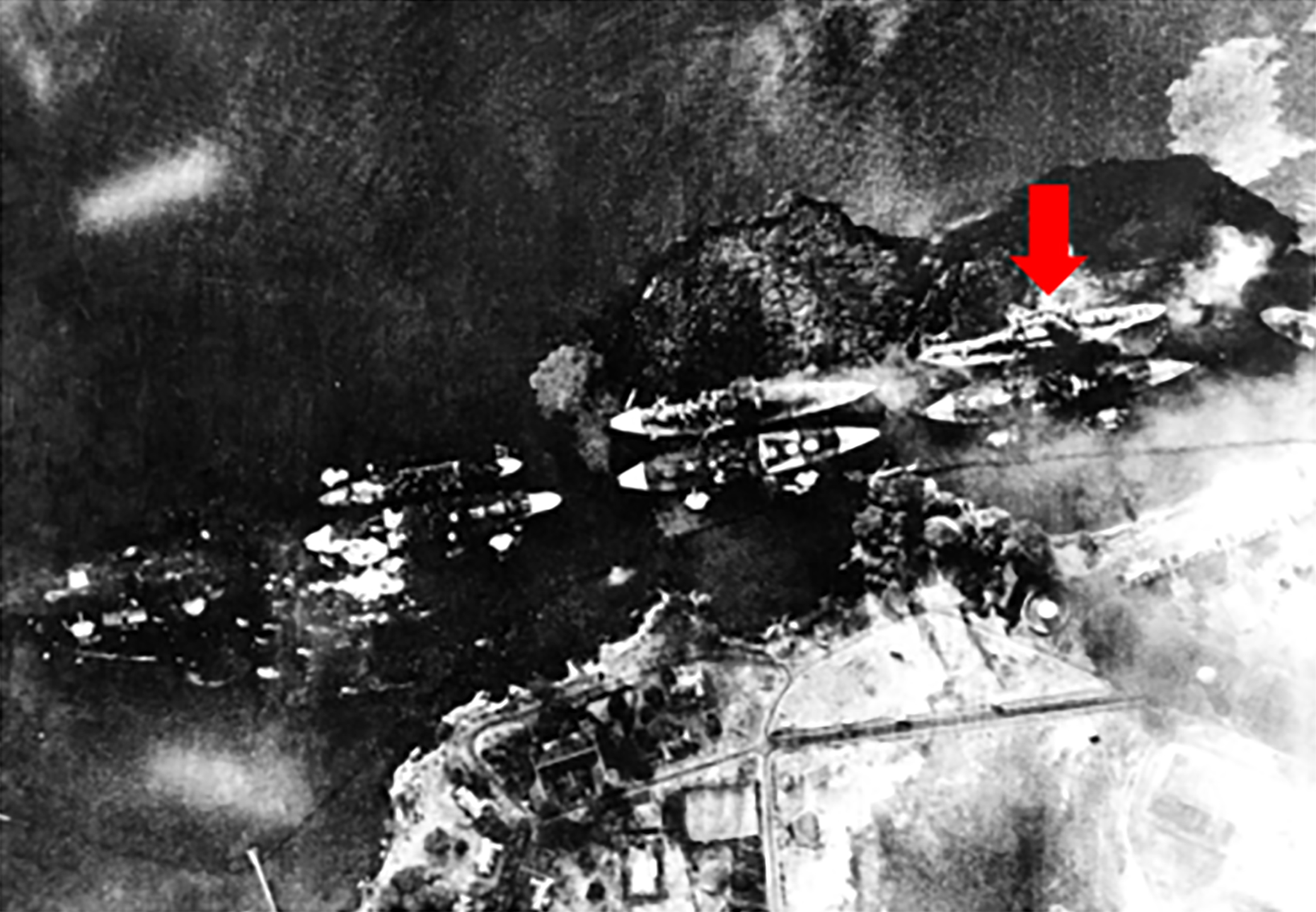
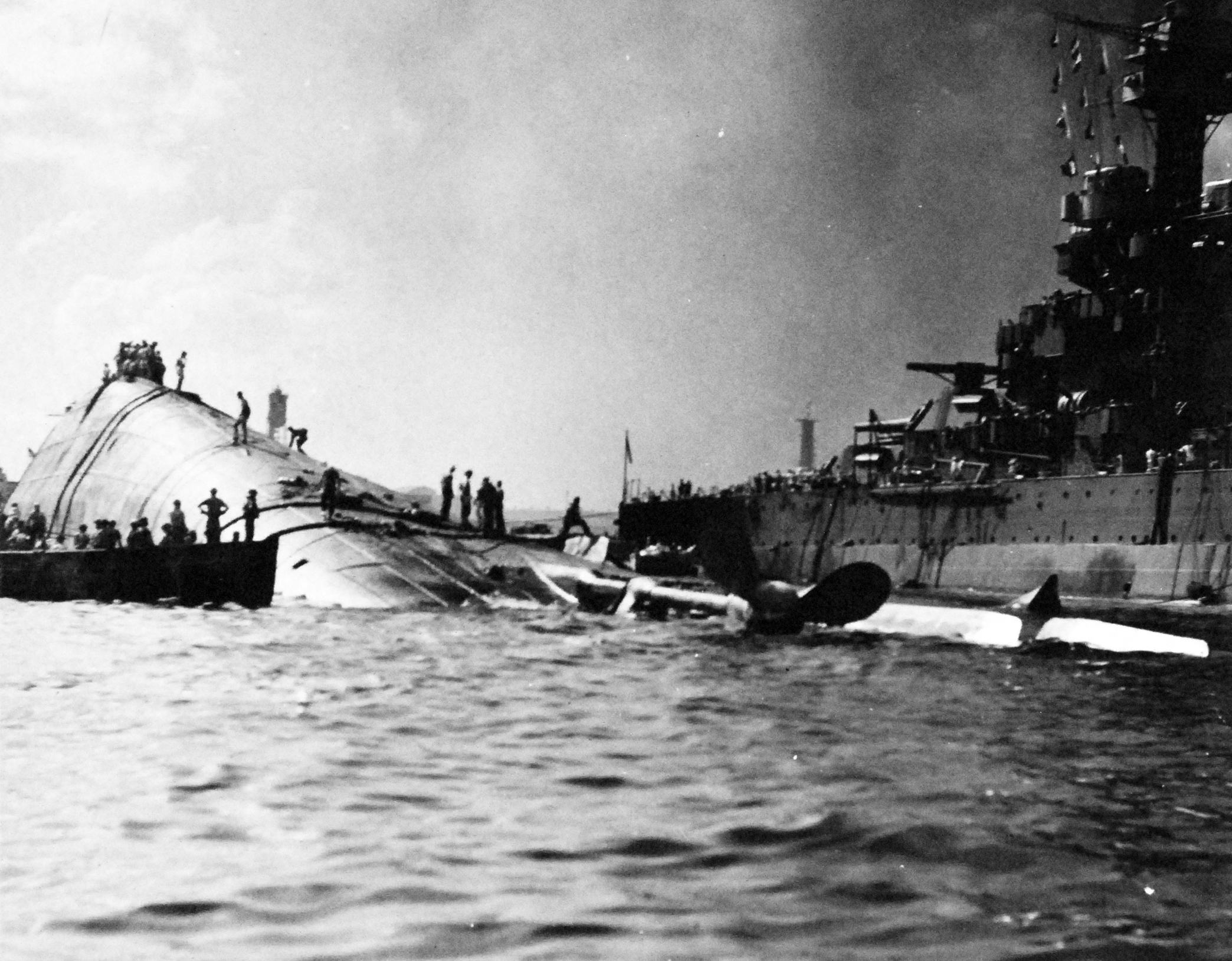
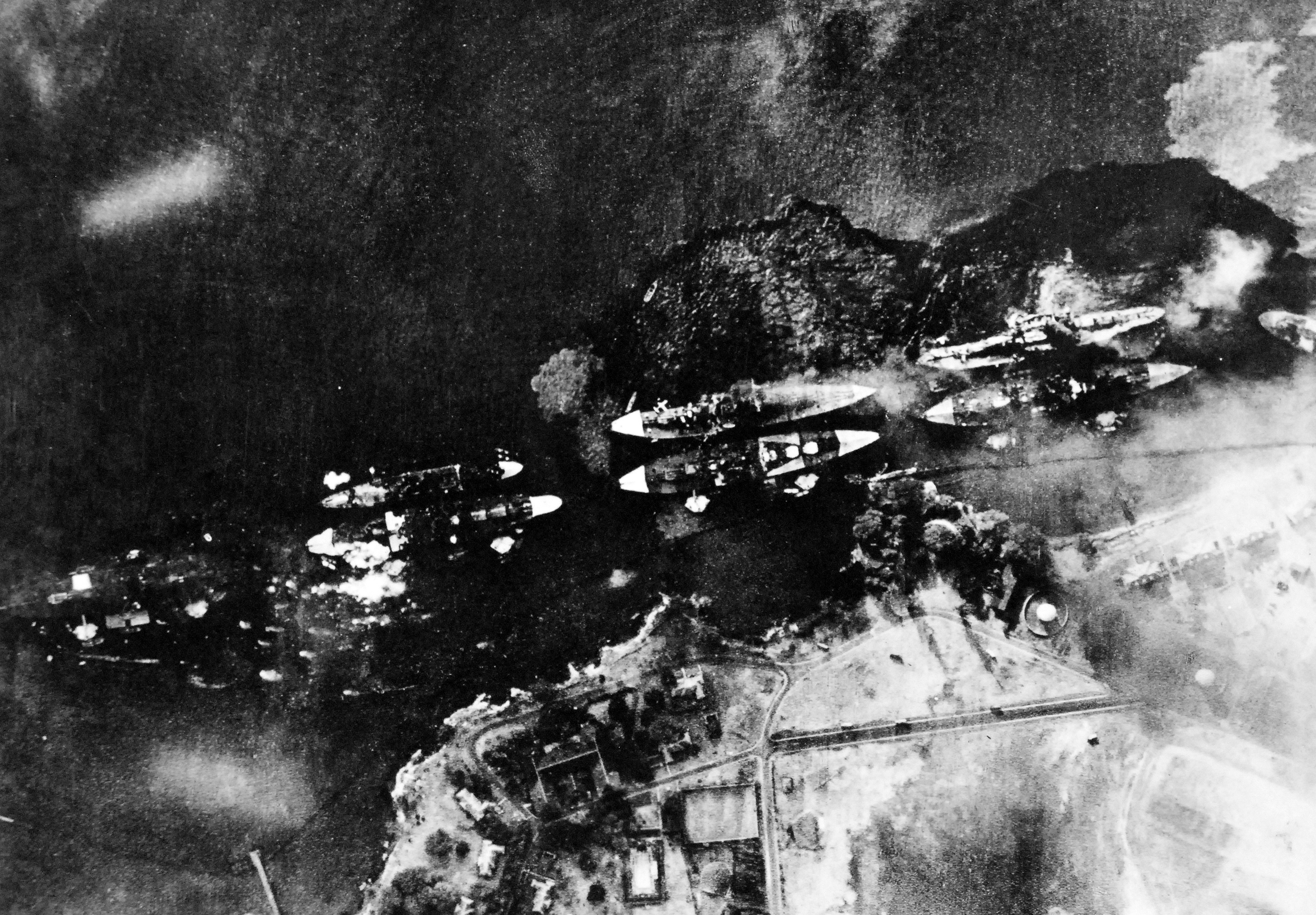
On 7 December 1941, the USS Oklahoma (BB-37)1 was hit by Japanese torpedoes during the attack on the U.S. Pacific Fleet in Pearl Harbor, Territory of Hawai’i (Fig. 1). The hits severely damaged the ship, which soon capsized (Fig. 2). The casualties, which included 429 individuals (415 U.S. Navy personnel and 14 Marines), represent the second-largest in the attack, after the USS Arizona.
Recovery efforts began the day following the attack, but they were halted on 16 December 1941. Salvage attempts began in July 1942 and continued until May 1944; during this time remains were also recovered (Harris 2010). The Oklahoma was decommissioned in September 1944, and while in transit to California in 1947 it sank again in the Pacific and was not recovered (Naval History and Heritage Command, no date). Ultimately, 35 individuals were identified in the years immediately following the attack, but the majority of the remains were buried as “unknowns” in two cemeteries on Oahu, Territory of Hawai’i—Nu’uanu and Halawa (Harris 2010).
Historical Analyses
In 1947, the American Graves Registration Service (AGRS) disinterred all Oklahoma unknowns from Nu’uanu and Halawa cemeteries. The remains were transferred to the Central Identification Laboratory at Schofield Barracks (Schofield CIL) to attempt individual identifications. However, the belief that the remains would ultimately be identified as a group assemblage drove analytical decisions and processes, including sorting the remains by element in order to bury them in as few caskets as possible.
FIG. 1—Aerial view of Battleship Row on December 7, 1941. The arrow indicates the position of the Oklahoma. Image available at http://navsource.org/archives/01/043/014303a.jpg.
FIG. 2—View of the capsized Oklahoma. Image available at http://navsource.org/archives/01/037/013741o.jpg.
When the request to bury the Oklahoma remains as a group was denied, analysts were tasked with reprocessing the remains in order to segregate the skeletal elements into individuals. Trotter (1949) reports that segregations were attempted based on articulation, size, color, morphology, and/or texture. These techniques were not enough to effectively segregate the commingled remains, and Dr. Trotter agreed to certify only the segregation of the cranial and/or mandibular remains of 27 individuals based on dental records (Harris 2010). She would not, however, certify any other segregations, including those of postcranial remains associated to the 27 crania/mandibles, due to her belief that the postcranial associations were not made in a scientifically sound manner (Harris 2010). The inability to segregate the remains into individuals for identification was likely due to the highly commingled nature of the assemblage and limitations of scientific techniques at the time, especially in the absence of DNA technology, and possibly also related to the demographic similarities of the decedent population.
The Office of the Quartermaster General, with oversight of AGRS, did not approve of these 27 cranial/mandibular segregations, as they felt that portions of these individuals could still be present in the commingled assemblage. Therefore, all disinterred Oklahoma unknowns were declared unidentifiable in 1949 and reburied as unknowns in 62 caskets within 46 graves at the National Memorial Cemetery of the Pacific (i.e., the Punchbowl) (Harris 2010). This left the number of unaccounted-for Oklahoma service members at 394.
Present-Day Analyses
The present-day analyses of the Oklahoma remains are divided into two time periods: 2003 to 2015 (pre-project) and 2015 to present (project).
2003 to 2015
Based on research conducted by a Pearl Harbor survivor, it was believed that a single casket buried in the Punchbowl contained the remains of five Oklahoma casualties (Harris 2010). The casualties in this casket were associated with Dr. Trotter’s work—specifically, segregations that she would not sign off on but felt that crania and/or mandibles could be reliably identified using dental records. The Joint POW/MIA Accounting Command (JPAC)—a predecessor to the present-day DPAA—agreed to disinter this casket in an attempt to identify the remains.
Ultimately, all five of the individuals who were believed to be in this casket were identified in the years following its disinterment, but a larger problem was revealed. In addition to the cranial remains of these five individuals, there were five “bundles” of remains containing postcranial elements. Each of these was associated with an Oklahoma “Unknown” number (X-number).2 Extensive DNA testing of nearly 200 of these elements indicated that 95 distinct mitochondrial DNA (mtDNA) sequences were present. In other words, the remains in the first casket represented a minimum of 25% of the Oklahoma casualties.
The disinterment of the remainder of the caskets was put on hold until the Department of Defense and other agencies could agree on a course of action. This included the need to collect DNA reference samples from Oklahoma families and compile relevant antemortem medical and dental records from unaccounted-for service members. Collection of reference samples included maternal relatives for mtDNA comparisons and relevant references for nuclear comparisons, to include paternal relatives for Y-chromosome short tandem repeat (Y-STR) testing and siblings and children for autosomal short tandem repeat (auSTR) testing. Self-references, especially for World War II cases, are extremely rare, and the DPAA identification process largely relies on mtDNA testing, with increasing use of nuclear testing as applicable and available.
In 2007 a single casket that was associated with Pearl Harbor losses but not a specific ship was disinterred from the Punchbowl. No commingling was detected, and this casket was quickly identified as a single Oklahoma loss.
On 14 April 2015 the Deputy Secretary of Defense approved the disinterment of the remaining 61 caskets associated with the Oklahoma (Work 2015). A timeline of five years was given to identify as many as possible of the 388 individuals carried as unaccounted-for following the previous decade’s efforts.
2015 to Present
Following the approval to disinter, remains were exhumed from the remaining 45 graves at the Punchbowl starting in June 2015. The exhumations were complete six months later, in November 2015. DNA sampling began in June 2015, and samples were sent to AFDIL on Dover Air Force Base, Delaware, where analyses began immediately.
The first identifications from the large-scale Oklahoma disinterment were made in September 2015, based on dental records. By April 2016 nearly 5,000 DNA samples had been taken and submitted to AFDIL for mtDNA sequencing. The number of samples submitted in 11 months represents a record for both the DPAA and AFDIL laboratories. One month later, in May 2016, the full inventory of the project was also completed (described below). During the sampling and inventory phase, identifications were also being made.
Analytical Procedures
Inventory
Upon accessioning, the remains in each casket were unpacked and cleaned by bundle at the DPAA Laboratory in Hawai’i, and each element was labeled with its X-number as a proxy for provenience. The remains were then repackaged and sent to the DPAA Laboratory in Nebraska, where analysts were assigned to conduct an inventory of the remains. Assignments were made by grave, also referred to as group number, so that the same analyst was responsible for the entire contents of a single grave. Since there were 62 caskets buried in 46 graves, some graves have two caskets while others have one. Inventory progressed through the groups in ascending order and included the first group from the casket disinterred in 2003.
The inventory process entails examining the remains by bundle, identifying and siding all elements, marking completeness using zones (Knüsel & Outram 2004), collecting data by element, assigning each element a unique designator (see below), and nominating samples for DNA testing. Some DNA samples were collected prior to the inventory process. Where this was the case, the samples taken were recorded and assessed; if additional samples were deemed necessary, the analyst nominated them. Data collection included: standard and supplemental measurements3 (Byrd & Adams 2003; Byrd & LeGarde 2014; Moore-Jansen et al. 1994);4 epiphyseal fusion and pubic symphysis component scores (McKern & Stewart 1957); antemortem trauma, to include fractures and pathologies; perimortem trauma; unique or otherwise potentially individuating characteristics (e.g., septal aperture); and taphonomic observations. These data were then entered into a single Excel spreadsheet.
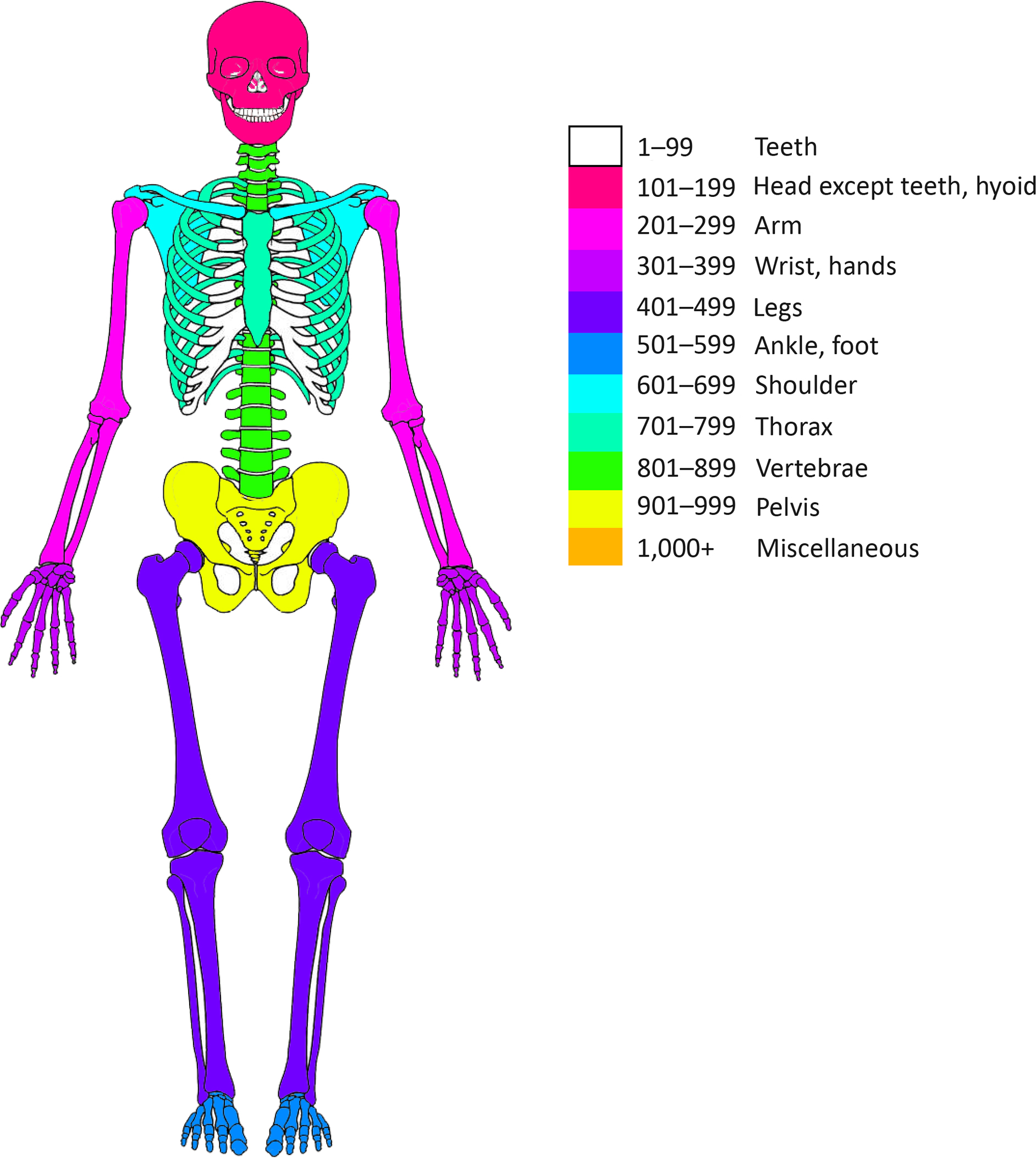
All elements were tagged with their unique designator—composed of the CIL case number, group number, X-number, and numerical designator by region of the body—using small paper tags with string or by adding the information to the DNA sampling tag. Numerical designators were by the hundreds, with each set of 100 representing a different body region (e.g., 200s are the arm; see Fig. 3). This system does not ascribe specific numbers to a specific bone, meaning that there is no empirical difference in 201 versus 299 within the 200s region, but it does allow for easy recognition of the region of origin of the element (i.e., 201 is not always a right humerus, but indicates a bone from the arm). Numbers are assigned in ascending order to elements within a particular region as they are encountered during inventory. This system was found to be particularly useful in the Oklahoma project, where the entire project was grouped under a single accession number and bundles contained duplicated elements, but the particular designator numbering scheme can be easily changed or adapted based on project context and scope.
Selection for DNA sampling first entailed an assessment of pair-matches and articulations within each bundle.5 This strategy allowed an analyst to nominate one or both paired bones based on their assessment of the pair within the bundle or nominate only one of several bones that articulate (e.g., vertebrae, pelvis). This strategy was not meant to replace larger scale comparisons of elements, but rather as a starting point for DNA sampling so that a limited sub-set of elements would be sampled since DNA sequencing is both time- and cost-prohibitive. The exception to the sampling strategy is the nomination of left and right humeri and tibiae regardless of pair-matching in order to collect data on historical and present-day pair-matching accuracy (see below and LeGarde 2019). All portions of the inventory process were peer-reviewed.
Segregation
Once the elements are sampled, the samples are sent to AFDIL for the first round of sequencing, which targets mtDNA hypervariable regions 1 and 2 (HVR1, HVR2). AFDIL produces a large Microsoft Excel spreadsheet that compares the polymorphisms of each sample for both HVR1 and HVR2 to all other samples in the project as well as all family reference samples (FRS) for the Oklahoma. This spreadsheet assigns a sequence number to each unique group of polymorphisms seen in the Oklahoma data set, and under each sequence number, all associated samples and service members are listed (i.e., those skeletal elements and FRS that have the same polymorphisms are listed under a single sequence number).
For the Oklahoma project, segregation of remains from the assemblage relies first on mtDNA sequence data due to the heavily commingled nature of the assemblage (see below) and then on anthropological associations such as pair-matching and articulation. An analyst is assigned work by mtDNA sequence, with two goals: 1. determine the number of individuals represented by the skeletal elements with the given mtDNA sequence and 2. associate non-sampled or not yet sequenced elements from the greater project assemblage. Additional nuclear DNA testing—Y-STR and auSTR—may be needed to aid in the segregation process, and analysts, along with the project lead, make recommendations to DPAA Laboratory management. Other regions of the mtDNA genome may be helpful for segregation (e.g., VR1, VR2), and upon AFDIL’s recommendation, elements also can be tested for these regions.
FIG. 3—Homunculus depicting the regional designator numbering scheme used for inventory.
Nuclear testing is not generally used as a first line of segregation at the DPAA Laboratory or in the Oklahoma project because of the success in sequencing mtDNA from the remains encountered by the DPAA Laboratory and because the majority of FRS are maternal. However, nuclear testing is useful when attempting to segregate sequences that have elements from two or more individuals. In these instances, when an analyst is unable to fully segregate multiple individuals in a given mtDNA sequence using anthropological methods such as visual pair-matching, articulation, and osteometric sorting (Byrd 2008; Byrd & Adams 2003; Byrd & LeGarde 2014), additional testing is requested to attempt to further separate remains. The type of testing requested is dictated by what references are available for service members associated via mtDNA and success rates of sequencing for the project as a whole. In the Oklahoma project, Y-STR testing is slightly more successful and there are more Y-STR FRS than auSTR FRS, so it is usually requested first.
Association of elements without DNA data is done by successfully pair-matching or articulating these elements to those yielding a specific mtDNA sequence. For pair-matching, the known element’s measurements are compared to all contralateral element measurements in the entire assemblage using an automated version of osteometric sorting (Byrd & Adams 2003; Byrd & LeGarde 2014; Lynch 2018a, 2018b; Lynch et al. 2018; also see below). Those elements that cannot be excluded as matching the known element based on measurements are then visually compared by the analyst, with potential morphological differences recorded on a diagram for the known specimen prior to comparison. If a potential match is identified, the morphology of the match is recorded on a second diagram, and the known specimen and potential match diagrams are compared for similarities. For articulations, generally only those with high reliability are examined and included in the absence of DNA data (e.g., pelvis, vertebrae; see Hines et al. 2014), and only those within the same original bundle are assessed. Occasionally, mandible-to-cranium articulations are employed to associate elements, but these associations are made only if the DPAA Laboratory odontologists agree.
Once the analyst has determined the number of individuals present and associated additional elements with those sequenced, elements are compared for size differences using osteometric sorting regression to ensure that all elements attributed to a single individual are consistent in size (Byrd & Adams 2003; Byrd & LeGarde 2014; Lynch 2018b). A segregation is complete once all elements have been attributed to discrete individuals and assigned an individual number (e.g., I-100). In cases where this is not possible, any remaining elements will be written up as non-attributable and remain in the parent sequence, rather than being assigned an individual number.
Segregation analysis is peer-reviewed in its entirety. Following peer review, a Forensic Anthropology Report (FAR) is written for each segregated individual. This report includes the biological profile, any noted antemortem or perimortem trauma, and any potentially individuating characteristics.
Association
The association process is the means by which a service member’s name is tied to a specific set of remains. For the Oklahoma, the results from the FAR are compared to the DNA results, dental records, and antemortem biological data in order to make a recommendation for identification to DPAA Laboratory management. At this point, additional nuclear testing (Y-STR or auSTR) may also be requested or employed in order to make or strengthen the association. The final association is only as strong as the antemortem data that are available for each service member.
The Sample
Antemortem Data
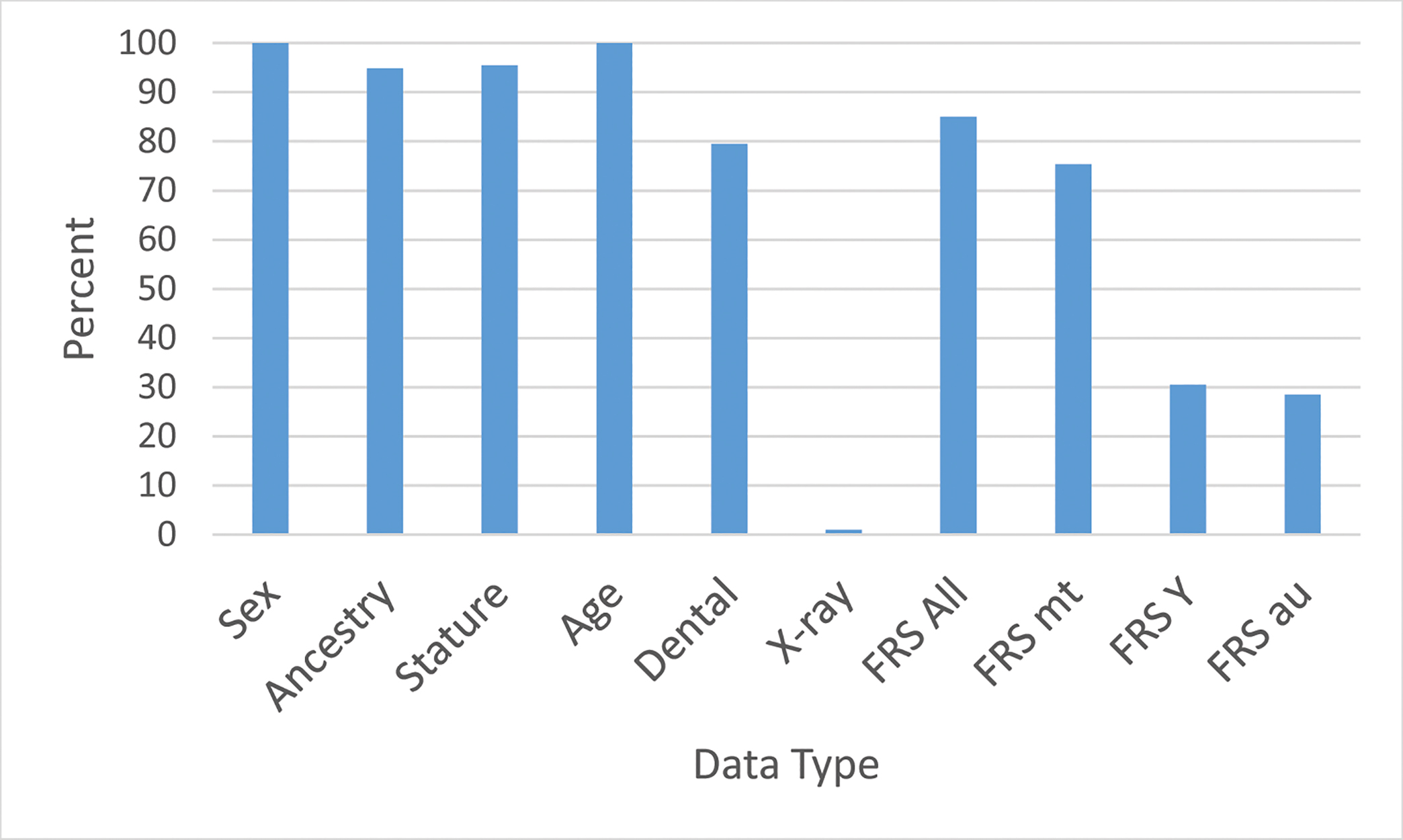
The available antemortem data for Oklahoma casualties are given in Figure 4. Antemortem biological data are drawn from military records and available for the majority of the Oklahoma casualties. All are adult males between the ages of 17 and 52 years at time of death, with a mean age of 24.5 years and a standard deviation of 6.4 years (n = 394). The mean stature is 68.6 inches, with a standard deviation of 2.3 inches (n = 376; unknown for 18 individuals). Military records indicate that 359 individuals are “White,” 12 individuals are “Black,” and 3 are “Asian (Pacific Islander)”; 20 are of unknown ancestry.
FIG. 4—Availability of antemortem data for Oklahoma casualties, expressed as percentages. A total for all DNA FRS is given (FRS All), and DNA is also divided by type (mtDNA, Y, autosomal).
DNA FRS are available for 85% of the casualties, though the numbers are different per DNA type (see Fig. 4). The most common FRS type is mtDNA. Only three individuals have chest radiographs on file, but due to the high success rate of mtDNA sequencing for the Oklahoma remains—nearly 99% of samples sequenced for mtDNA to date have yielded results—this line of evidence has not yet contributed to an Oklahoma identification.6
Dental records are available for just under 80% of the casualties, but the strength of this line of evidence varies among the service members. For example, when only induction records are available, they are more useful for an individual with an age at death of 18 versus someone with an age at death of 52, since a greater amount of time has passed between the dental exam and death. A greater amount of time between exam and death means that potentially more dental work could be present but not recorded, which presents challenges for associating dental remains with one service member over another.
Postmortem Data
The Oklahoma assemblage consists of nearly 13,000 skeletal elements buried in 392 distinct bundles. This number includes both identifiable elements and unidentifiable fragments, although nearly 90% of the elements are both identifiable and complete. Fragmentation of the elements is minimal, and preservation is excellent.
Of the 62 caskets, 60 contained two or more bundles. For these 60 caskets and 390 bundles, on average, there were 8.9 bundles per casket and 32.1 elements per bundle, with a minimum of 4 and a maximum of 175 elements per bundle. These numbers do not include teeth or unidentified fragments.
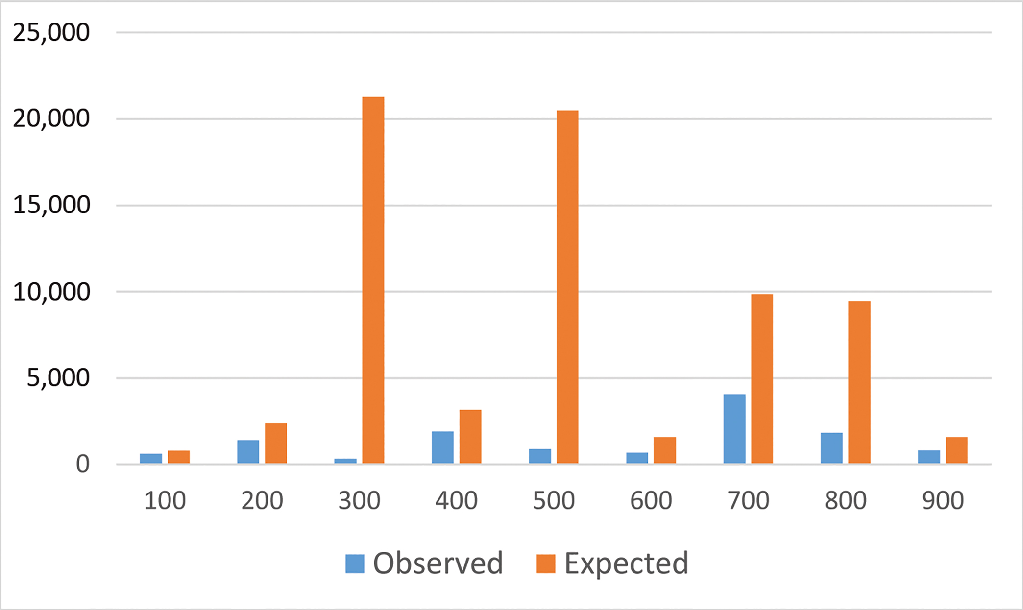
The MNI represented by the assemblage using the most numerous duplicated element (cranium) is 357, though the thorax (700; ribs and sternum) has the highest total number of elements recovered (Fig. 5). When combining mtDNA sequences and skeletal duplication (i.e., the most numerous element for a particular sequence gives the MNI for that sequence; all individual MNI tabulations by sequence are then totaled across the assemblage), the MNI increases to 400. See Palmiotto et al. (2019) for a more detailed discussion of estimating the number of individuals in this assemblage.
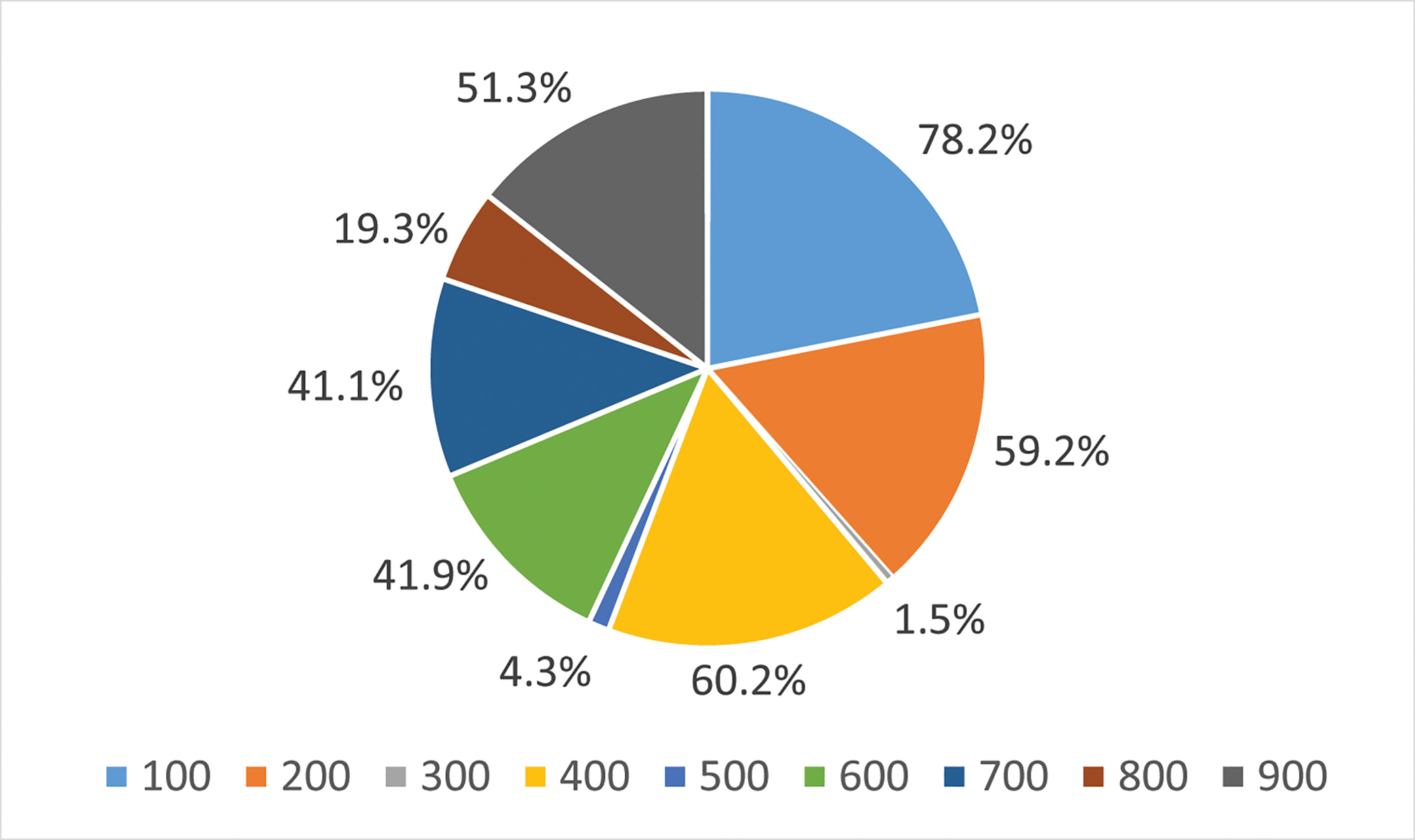
Elements are not represented equally. Figures 5 and 6 provide data on differences in recovery rate for elements by region; Table 1 lists what elements are considered in these counts. The expected number of elements is calculated by multiplying the number of unaccounted-for individuals (394) by the number of elements in a particular series (e.g., 200 [arm] = 6). While this does not take into account potential pairs or refits of fragmented elements, this calculation provides an easy comparison in terms of assemblage composition. It is important to note that observed totals do not approach expected totals even for the most numerous region (thorax), indicating that the number of elements recovered is always much less than what would be expected (see Fig. 5). Note that recovery rates for the hands (300) and feet (500) are especially low, while the recovery rate for the head (100) is the highest, followed by the arms (200) and legs (400).
FIG. 5—Count of elements by region, comparing observed and expected.
FIG. 6—Ratio of elements observed to expected, by region.
TABLE 1—Elements Used for the Comparison of Observed versus Expected Elements in the Oklahoma Assemblage.
|
Region |
Elements |
|
|
100 |
Cranium, mandible |
|
|
200 |
Humerus, radius, ulna |
|
|
300 |
Carpals, metacarpals, manual phalanges |
|
|
400 |
Femur, patella, tibia, fibula |
|
|
500 |
Tarsals, metatarsals, pedal phalanges |
|
|
600 |
Clavicle, scapula |
|
|
700 |
Ribs, sternum |
|
|
800 |
Vertebrae |
|
|
900 |
Innominate, sacrum, coccyx |
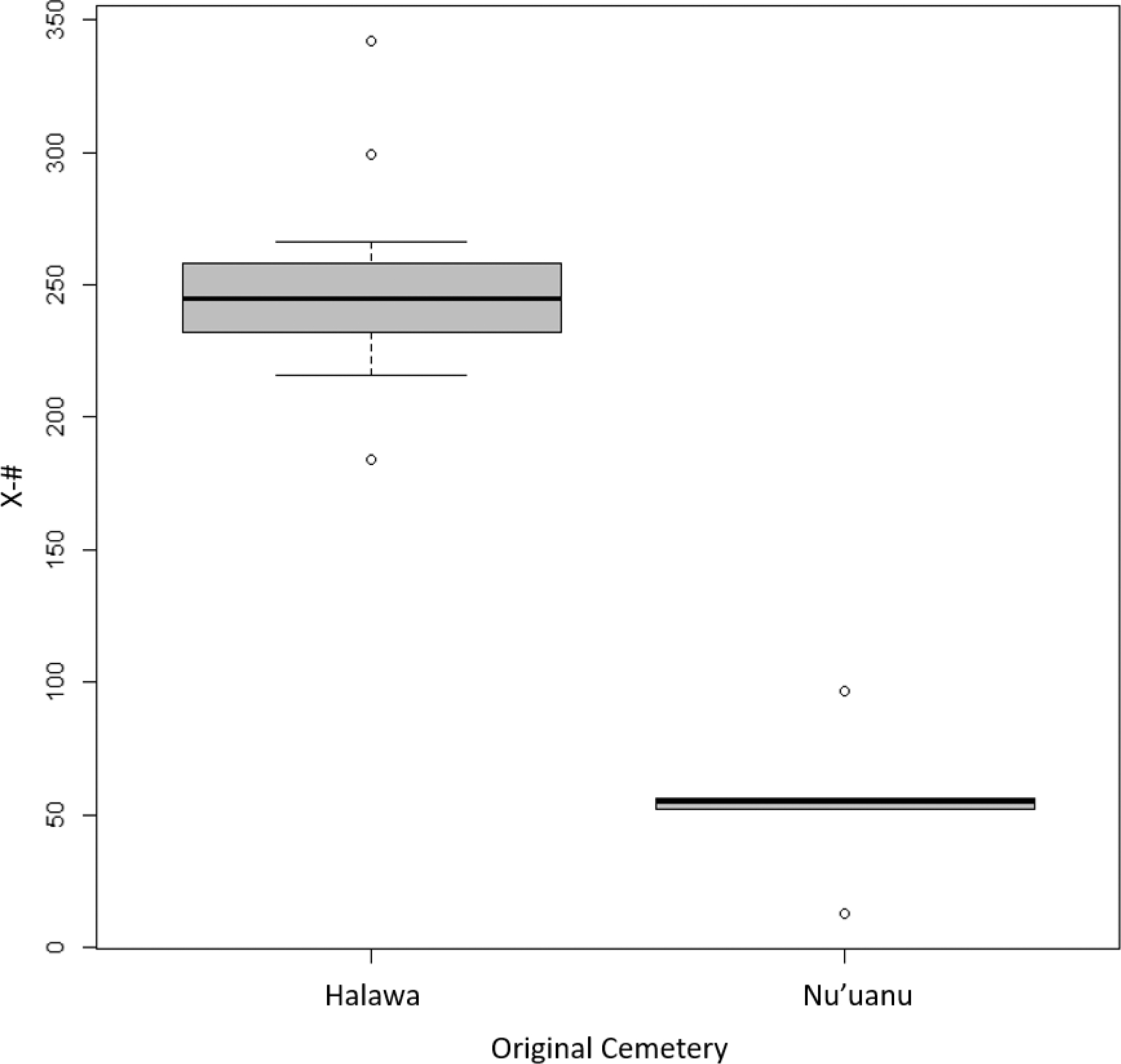
When examining the remains in terms of potential provenience information (i.e., X-number), there is a difference in terms of what X-numbers were originally buried in Nu’uanu versus Halawa prior to the 1947–1949 processing (Fig. 7). All X-numbers less than 100 were originally buried in Nu’uanu cemetery, while those greater than 100 were buried in Halawa. It might then be expected that individuals recovered first and buried in Nu’uanu would be less commingled than those recovered later and buried in Halawa. Yet, the results seen thus far suggest that the commingling that occurred during the reprocessing efforts does not seem to have occurred within only one cemetery group (i.e., elements from X-numbers less than and greater than 100 are commingled together).
FIG. 7—Relationship of X-number (bundle) to original cemetery.
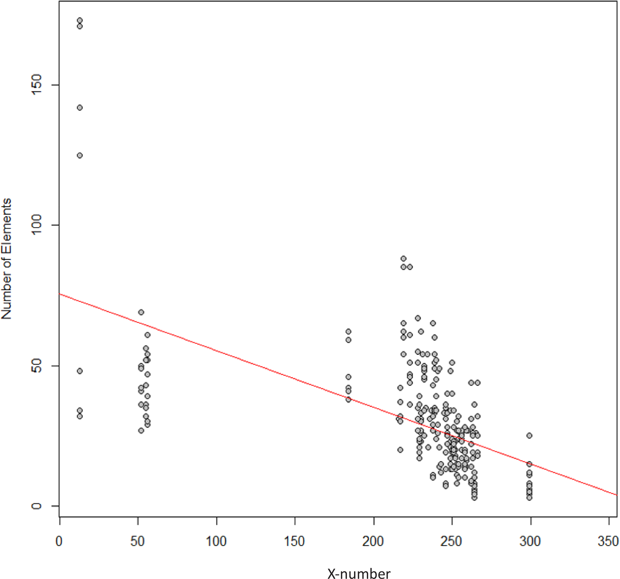
FIG. 8—Relationship of X-number (bundle) to the number of elements in the bundle representing it.
Given the extensive commingling noted in this assemblage, it is interesting that there is still a negative correlation between the X-number and the number of elements in the bundle representing it (Fig. 8); a higher X-number is associated with fewer elements. This makes sense in terms of recovery efforts in the 1940s, since X-numbers were assigned in ascending order, and those remains recovered earlier are likely to have more elements than those recovered months and years post-incident. However, given the reprocessing that occurred from 1947 to 1949 it is unclear why the relationship still holds true today, since presumably all elements were equally commingled during the reprocessing phase in the 1940s, especially given what is known about the extreme commingling across the entire assemblage (see below). It is possible that X-numbers were reassigned during the reprocessing phase, so that those remains that were more complete were given lower X-numbers. If this is the case, the X-numbers are virtually meaningless in terms of aiding in present-day segregations given what is known about how great the commingling is.
Extent of Commingling
Based on the mtDNA results from the first casket, where 25% of the Oklahoma casualties are represented by at least one skeletal element, it was expected that commingling was extreme. Disinterment of the remainder of the caskets confirms this. With the exception of two caskets, multiple bundles are present in each casket, and none of these bundles contain elements from a single individual. Conversely, no individual identified to date has skeletal elements from only a single bundle or even a single casket.
A preliminary investigation of historical element associations within bundles confirms Dr. Trotter’s fears that segregations were being made arbitrarily, at least in part (Brown et al. 2017). Using mtDNA results, Brown et al. (2017) found that the humeri and tibia are correctly associated to their antimeres 44% and 46% of the time, respectively, but only 6% of the time when humeri are compared to tibiae in the same bundle. While the pair-matching numbers may seem low, it is important to remember that the comparisons undertaken were on the order of 100,000 given the presence of approximately 300 elements of each side for both the humeri and tibiae. Thus an accuracy of 50% may represent the best-case scenario historically given the limitations of methods 70 years ago. However, 6% likely represents nothing more than chance.
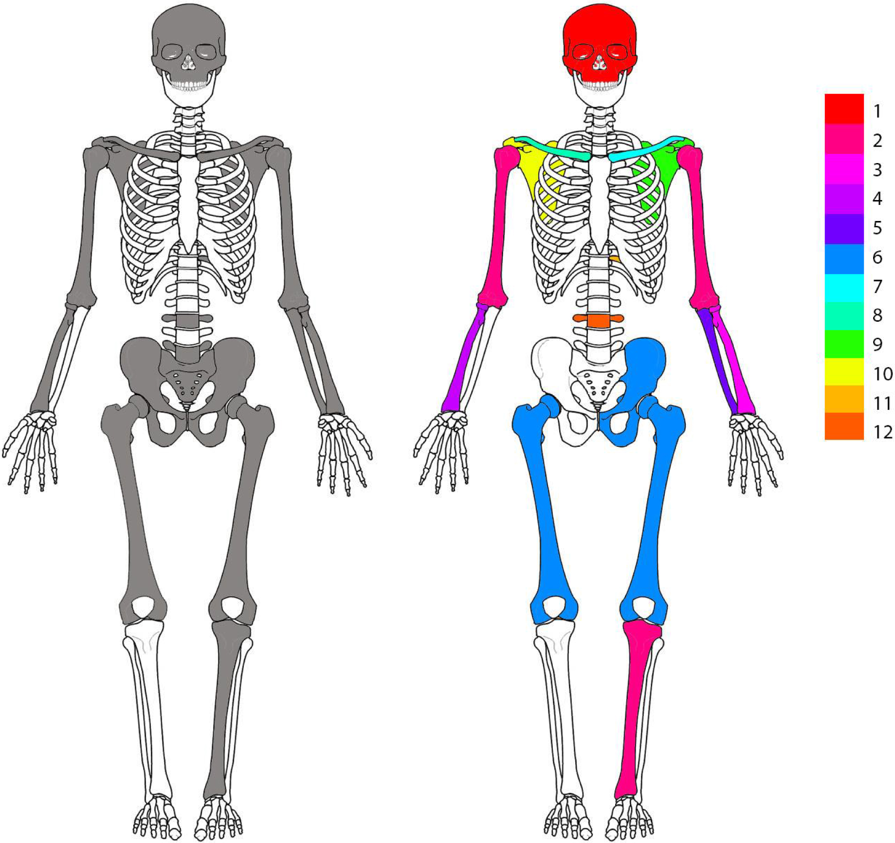
Figures 9 and 10 demonstrate the extent of commingling; Figure 9 depicts a single bundle, and Figure 10 depicts an identified individual. In Figure 9, the initial by-element inventory on the left does not indicate commingling when just element duplication is considered. However, when mtDNA sequences are overlaid, 12 different sequences are seen. Thus, a bundle that appears on first glance to be a single individual actually represents portions of at least 12 individuals, and likely more given that not all elements are sampled and the rarity of the mtDNA sequence is not considered here.7
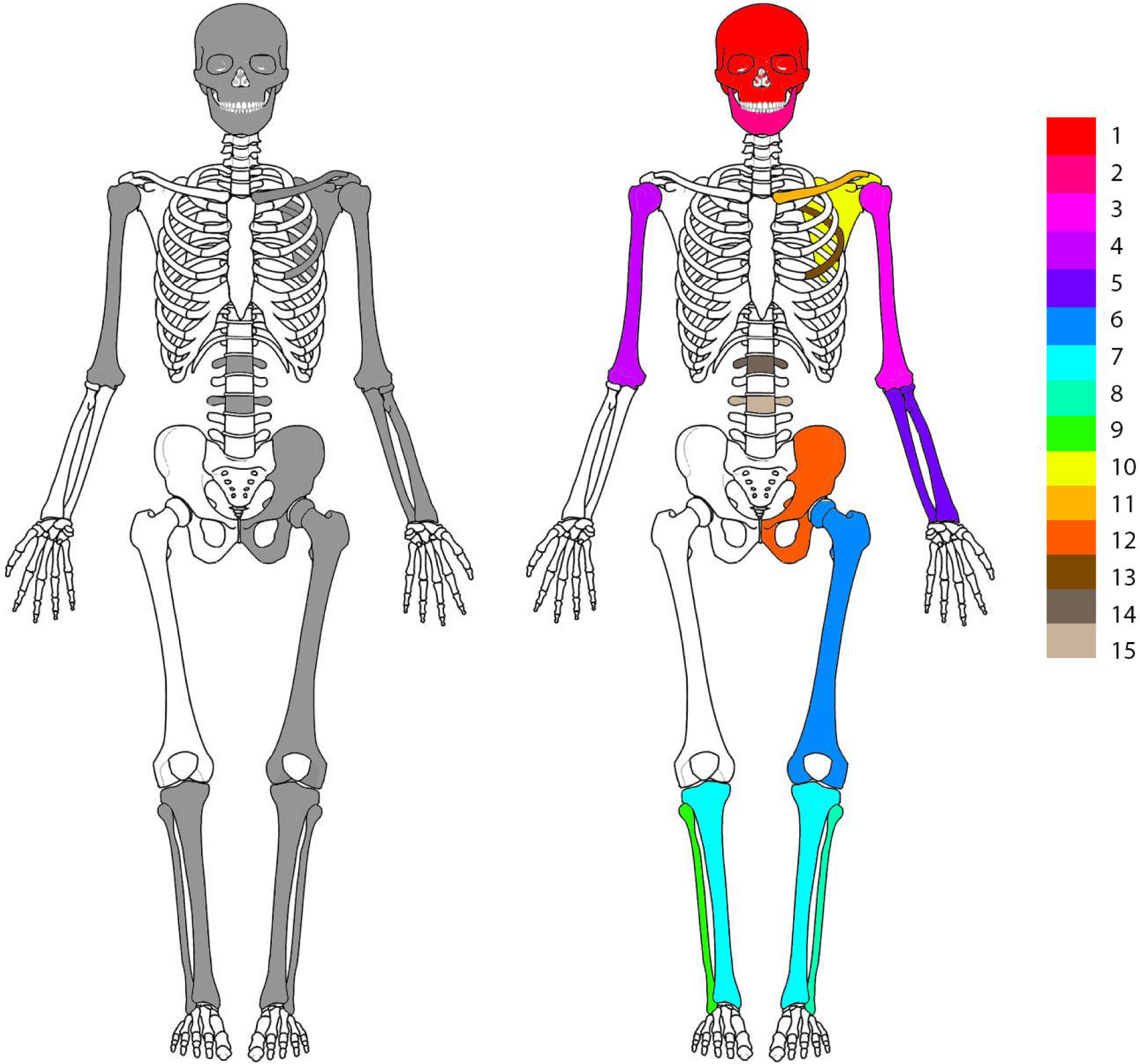
In Figure 10, that of an identified individual, all skeletal elements are from the same mtDNA sequence, but this time the origin of the elements by bundle (X-number) is depicted. For this individual, who has 17 elements present, 15 came from different bundles. Notably, the cranium/mandible and innominate/femur have different sequences, which may speak to the lack of reliability of these articulations for association. Both the historical tibia pair-match and the radius-ulna articulation were correct in isolation but were not correct in terms of association to a single individual.
FIG. 9—Homunculi depicting a single bundle of remains. Left, initial by-element inventory with no skeletal duplication; right, elements sampled with sequences indicated. The homunculus on the right does not include elements articulated or pair-matched. Note: multiple ribs are present, but only the one sampled is depicted; the teeth are not depicted.
FIG. 10—Homunculi depicting an identified individual. Left, all elements present in a single mtDNA sequence with a single match to an Oklahoma FRS; right, element provenience (X-number) indicated. Note: the teeth are not depicted.
While not all DNA samples have been sequenced, thus far the data indicate that, on average, commingling is around 80% per bundle. That means that for every 10 elements sequenced in a bundle, 8 will return a different mtDNA sequence. Thus using a bundle as a true provenience is not possible, and there appears to be no true relationship among elements in any given bundle.
Identifications
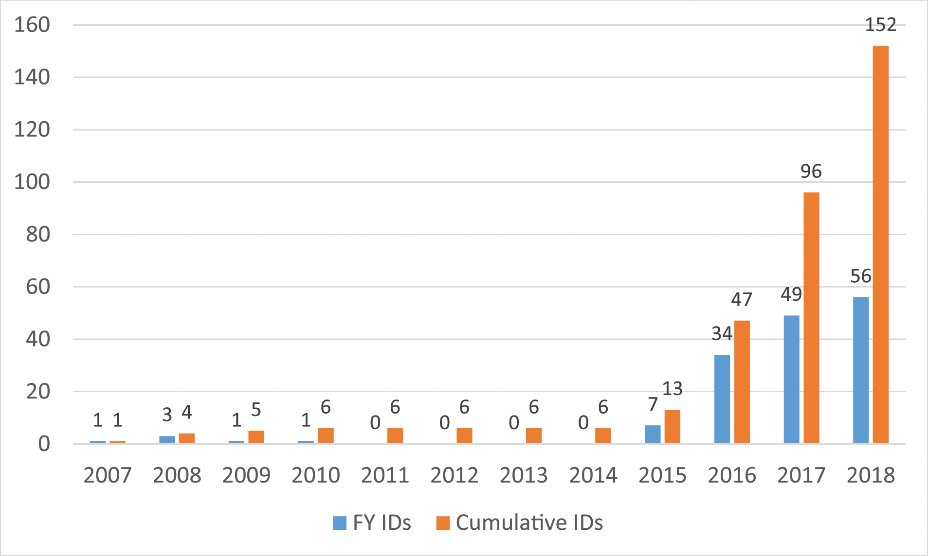
Oklahoma identifications are made using a combination of DNA, dental, and anthropological analyses. As of 9 August 2018, 152 identifications had been made (Fig. 11). This means that three years following the disinterment of the majority of Oklahoma caskets, 35% of the individuals who were unaccounted for following World War II have been identified.
Identifications have been made in three phases: pre-project (2003 to 2010), initial project (September 2015 to April 2017), and project (July 2017 to present) (see Fig. 11). The identifications made prior to the project were those from the initial 2003 Oklahoma casket and the single 2007 Pearl Harbor–associated casket. The five identifications from the 2003 disinterment were cranial/mandibular only, and therefore it is expected that there will be postcranial portions of these individuals commingled with remains from other caskets. The 2007 identification represents a complete set of remains, so it is not expected that commingling of this individual will be seen in the larger Oklahoma assemblage. The initial project identifications relied largely on dental identifications, with some support from DNA. During this phase, only crania and/or mandibles were identified. Like five of the individuals from the pre-project identifications, it is expected that additional remains will be associated with these individuals as the project progresses.
FIG. 11—Oklahoma identifications by fiscal year (FY). The DPAA FY runs from 1 October to 30 September. Note the uptick in identifications following the exhumations in 2015 and the increasing pace of identifications in 2018 due to receipt of increased numbers of mtDNA results. Data as of 9 August 2018.
Project identifications include cranial and postcranial remains. These cases are worked fully by the Oklahoma team and are presented to DPAA Laboratory management, including the DPAA Medical Examiner (ME), and AFDIL on a regular basis. Once DPAA Laboratory management and the ME agree on the association proposed by the team, the case moves forward for identification. Identifications are made by the DPAA ME, and families are notified by the respective Service Casualty Office. For the Oklahoma this is the Navy and the Marine Corps.
Challenges
Beyond the extensive commingling, additional challenges were encountered during the inventory and analysis of the Oklahoma assemblage. Due to the size of the assemblage, data management and analysis became increasingly difficult in terms of data integrity, access, and scale of comparisons as inventory and analysis progressed.
The project was initially inventoried on paper forms and then data were entered into a Microsoft Excel spreadsheet. This worked relatively well when only one person was working on data entry, but as the project team grew it became very difficult to continue, since Excel only allows one individual access at a time. Attempts to work in different spreadsheets and merge them together were not successful, and data were often inadvertently deleted, moved, or altered. Using Microsoft Access did not fix these issues, and a more sophisticated option was envisioned.
The Commingled Remains Analytics (CoRA) multi-user web application was developed in a partnership with the University of Nebraska at Omaha’s College of Information Science and Technology. This application enables by-element inventory; biological profile, trauma, and taphonomy data collection; assignment and DNA tracking; and overall project management for commingled remains. The hope for future development of CoRA includes the ability to integrate other anthropology applications (e.g., FORDISC, OsteoSort). Currently, CoRA is only available for internal use by DPAA, but it is anticipated that it will be released in the future for public use. Additional information about CoRA can be found at https://cora-docs.readthedocs.io/en/latest/.
Comparisons of elements across the Oklahoma assemblage also presented a challenge. With major long bones numbering around 300 for each side, pairwise comparisons for a single element were over 100,000 and precluded by space and time. In order to harness the power of osteometric sorting, OsteoSort was developed to automate the association process (Lynch 2018a, 2018b; Lynch et al. 2018). OsteoSort is available online at https://osteocoder.com/, and online applications include single pairwise comparisons, articulations, and regression analyses as well as antemortem stature comparisons to maximum length measurements. If multiple element comparisons are desired, OsteoSort can also be run in the statistical package R (R Core Team 2014). More information about OsteoSort is available on the above-cited website.
Conclusion
The Oklahoma assemblage provides unique opportunities to better our understanding of techniques used to resolve commingling, as well as insight into historical forensic anthropological investigations. Because the elements are largely complete and well preserved, the assemblage offers an excellent opportunity to research current methods and develop new ways of analyzing commingled remains. It is anticipated that in addition to the research in this issue, further research on recovery rate, MNI, age estimation, osteometric sorting, and reliability of articulations will be conducted, especially once DNA sequencing is complete.
References
Brown CA, LeGarde CB, Damann FE, Byrd JE. Assessing the accuracy of historical associations in a commingled assemblage. In: Proceedings of the 69th Annual Meeting of the American Academy of Forensic Sciences, February 13–18, 2017; New Orleans, LA.
Byrd JE. Models and methods for osteometric sorting. In: Adams BJ, Byrd JE, eds. Recovery, Analysis, and Identification of Commingled Human Remains. Totowa: Humana Press; 2008:199–220.
Byrd JE, Adams BJ. Osteometric sorting of commingled human remains. Journal of Forensic Sciences 2003;48(4):717–724.
Byrd JE, LeGarde C. Osteometric sorting. In: Adams BJ, Byrd JE, eds. Commingled Human Remains: Methods in Recovery, Analysis, and Identification. San Diego: Academic Press; 2014:167–191.
Harris H. History of the sinking of USS Oklahoma and subsequent attempts to recover and identify her crew. March 1, 2010. http://www.public.navy.mil/bupers-npc/support/casualty/Documents/POW%20MIA/USS%20OKLAHOMA%20(BB-37).pdf. Accessed June 1, 2018.
Hines DZC, Vennemeyer M, Amory S, Huel RLM, Hanson I, Katzmarzyk C, et al. Prioritized sampling of bone and teeth for DNA analysis in commingled cases. In: Adams BJ, Byrd JE, eds. Commingled Human Remains: Methods in Recovery, Analysis, and Identification. San Diego: Academic Press; 2014:275–305.
Knüsel CJ, Outram AK. Fragmentation: The zonation method applied to fragmented human remains from archaeological and forensic contexts. Environmental Archaeology 2004;9:85–98.
Langley NR, Jantz LM, Ousley SD, Jantz RL, Milner G. Data collection procedures for forensic skeletal material 2.0. University of Tennessee, Knoxville; 2016
LeGarde CB. Preliminary findings from a visual pair-matching study in a large commingled assemblage. Forensic Anthropology 2019;2(2):65–71.
Lynch JJ. An analysis on the choice of alpha level in the osteometric pair-matching of the os coxa, scapula, and clavicle. Journal of Forensic Sciences 2018a;63(3):793–797.
Lynch JJ. The automation of regression modeling in osteometric sorting: An ordination approach. Journal of Forensic Sciences 2018b;63(3):798–804.
Lynch JJ, Byrd JE, LeGarde CB. The power of exclusion using automated osteometric sorting: Pair-matching. Journal of Forensic Sciences 2018;63(2):371–380.
McKern TW, Stewart TD. Skeletal age changes in young American males analyzed from the standpoint of age identification (QREC-EP-45) Natick, MA: Quartermaster Research and Engineering Command; 1957.
Moore-Jansen PM, Ousley SD, Jantz RL. Data collection procedures for forensic skeletal material. Report of Investigations No. 48. University of Tennessee, Knoxville; 1994.
Naval History and Heritage Command. USS Oklahoma (Battleship # 37, later BB-37), 1916–1946, https://www.history.navy.mil/our-collections/photography/us-navy-ships/battleships/oklahoma-bb-37.html. Accessed June 1, 2018.
Palmiotto A, Brown CA, LeGarde, CB. Estimating the number of individuals in a large commingled assemblage. Forensic Anthropology 2019;2(2):129–138.
R Core Team. R: A language and environment for statistical computing. R Foundation for Statistical Computing, Vienna, Austria, 2014. http://www.R-project.org/.
Stephan CN, Winburn AP, Christensen AF, Tyrrell AJ. Skeletal identification by radiographic comparison: Blind tests of a morphoscopic method using antemortem chest radiographs. Journal of Forensic Sciences 2011;56(2):320–322.
Trotter M. Operations at Central Identification Laboratory. 1949. http://beckerexhibits.wustl.edu/mowihsp/words/TrotterReport.htm. Created 2004. Accessed June 4 2018.
Work RO. Memorandum for Secretaries of the Military Departments, et al. Subject: Disinterment of Unknowns from the National Memorial Cemetery of the Pacific. April 14, 2015. https://www.defense.gov/Portals/1/Documents/pubs/DSD_Memo_Disinterment_of_Unknowns_from_the_National_Memorial_Cemetery_of_the_Pacific.pdf.
1. Following the U.S. Navy hull classification system, BB = battleship, 37 = hull number. Navy ships are identified by type of ship and unique hull number within that type.
2. X-numbers were assigned to cases that could not be identified and were most commonly assigned by cemetery, forming a two-part numbering system (e.g., Nu’uanu X-97). The Oklahoma X-numbers were assigned in ascending order based on order of recovery (i.e., a lower number indicates remains that were recovered earlier). However, based on the processing that occurred from 1947 to 1949, it is doubtful that the X-numbers are truly meaningful for individual elements.
3. A list of measurements and their descriptions can be found at https://cora-docs.readthedocs.io/en/latest/forensics-anthro-guide/measurements/. A measurement guide that standardizes the numbering systems across multiple methods is available at https://osteocoder.com/wp-content/uploads/2018/04/Standardized_Measurements.pdf.
4. At the time data collection started for the Oklahoma project, the updated data-collection procedures (Langley et al. 2016) had not yet been released, so all measurements were taken following the Moore-Jansen et al. (1994) standards for consistency throughout the duration of the project.
5. Bundles are assumed to be historical representations of individuals, that is, the most parsimonious associations of elements made during the reprocessing efforts in the late 1940s.
6. The method of radiographic comparison using chest radiographs is employed by the DPAA Laboratory because of challenges in obtaining DNA from certain cases. This method compares a service member’s antemortem chest radiograph to the remains present (clavicles, lower cervical vertebrae, and upper thoracic vertebrae) to make an identification (Stephan et al. 2011).
7. Rarity of the sequence is determined by AFDIL and is given as the number of times a group of polymorphisms is seen in the AFDIL population database (n = 10,428). For the Oklahoma project, rarity ranges from 0 to 360 out of 10,428.
aDefense POW/MIA Accounting Agency—Laboratory, Offutt AFB, NE, USA
*Correspondence to: Carrie Brown, Defense POW/MIA Accounting Agency—Laboratory, 106 Peacekeeper Dr., Bldg. 301, Offutt AFB, NE 68113-4006, USA
e-mail: carrie.a.brown40.civ@mail.mil
Received 14 June 2018; Revised 13 August 2018; Accepted 30 August 2018