Forensic Anthropology Vol. 2, No. 2: 72–86
DOI: 10.5744/fa.2019.1000
RESEARCH ARTICLE
A Novel Method for Osteometric Reassociation Using Hamiltonian Markov Chain Monte Carlo (MCMC) Simulation
ABSTRACT: Traditional osteometric reassociation uses an error-mitigation approach, which seeks to eliminate possible matches, rather than a predictive approach, where possible matches are directly compared. This study examines the utility of a Bayesian approach for resolving commingling by using a probabilistic framework to predict correct matches.
Comparisons were grouped into three types: paired elements, articulating elements, and other elements. Ten individuals were randomly removed from the total sample (N = 833), acting as a small-scale, closed-population commingled assemblage. One element was chosen as the independent variable, with the ten possible matching elements representing the dependent variable. A Bayesian regression model was constructed using the remaining total sample, resulting in a distribution of possible values that were smoothed into a probability density, and probabilities were calculated. The element with the highest posterior probability was considered the best match. This process was repeated 500 times for each comparison. The correct match was identified 51.60% of the time. Paired elements performed the best, at 80.76%, followed by 42.10% for articulating and 33.63% for other comparisons.
These results suggest that metric analysis of commingled assemblages is complex and that both elimination-based and prediction-based approaches have a role in resolving commingling. In this regard, the strength of a Bayesian approach is versatility, allowing for prediction of the correct match and elimination of possible matches, as well as integration of independent lines of evidence within one cohesive model.
KEYWORDS: forensic anthropology commingling, Bayesian modeling, MCMC simulation
Introduction
In osteological analysis, commingled assemblages present a situation in which discrete sets of remains are not readily apparent. Commingled assemblages, such as ossuaries, are a fairly common situation in bioarchaeology (Curtin 2008; Herrmann & Devlin 2008; Ubelaker & Rife 2008; Willey 1990). With the increasing utilization of forensic anthropologists in arenas such as mass disaster (Hinkes 1989; Mundorff 2008, 2012; Sledzik & Rodriguez 2001), cremation litigation (Steadman et al. 2008), and human rights investigations (Primorac et al. 1996; Varas & Leiva 2012), resolution of commingling is becoming commonplace (Adams & Byrd 2008, 2014). Forensic analysis of commingled remains focuses on victim identification and reassociating remains into discrete individuals (Adams & Byrd 2006, 2008, 2014; Byrd & Adams 2003, 2009). This focus has led to an increase in research on methodology for resolving commingling (Adams & Byrd 2008, 2014).
Of the methods available for resolving commingling, osteometric reassociation, which uses statistical models to compare bone dimensions, is considered a reliable and relatively objective technique (Adams & Byrd 2006; Buikstra et al. 1984; Byrd 2008; Byrd & Adams 2003; Byrd & LeGarde 2014; Konigsberg & Frankenberg 2013; O’Brien & Storlie 2011; Rosing & Pischtschan 1995; Snow & Folk 1970). Traditional osteometric sorting logic is a decision-making, error-mitigation approach (Byrd 2008; Byrd & Adams 2003; Byrd & LeGarde 2014). This approach does not seek to reassociate elements per se; rather the analyst tests the null hypothesis that the dimensions of two bones are similar enough to have derived from the same individual (Adams & Byrd 2006; Byrd 2008; Byrd & Adams 2003; Byrd & LeGarde 2014). Possible matches are eliminated if the calculated p-value exceeds an analyst-defined threshold, or alpha level. Bones are reassociated if all other possible matches can be eliminated. This approach implies that, because of broad variation in intra-individual bone size, reassociation is achievable via osteometrics when the assemblage represents a closed population of a smaller number of different-sized individuals (Byrd 2008).
The logic of reassociation through elimination was first introduced by Byrd and Adams (2003). A regression model and associated 90% prediction interval, based on the natural logarithm of the summed measurements by element, was constructed. If the bone in question fell outside of the 90% prediction interval, the researcher concluded that the elements are too different in size to be from one individual. The form of decision making used by Byrd and Adams (2003) follows a Neyman-Pearson approach to hypothesis testing, where decisions concerning the null hypothesis are strictly based on whether a test statistic passes an a priori threshold value (Royall 2000). The researcher is making a dichotomous decision whether to reject or fail to reject the null hypothesis. Under this paradigm, there is no degree of belief in the null hypothesis—it is either rejected or it is not (Royall 1997). The explicit decision-making rationale and ease of interpretation of this approach to science has obvious strengths. The elements in question either derive from the same individual or they do not; there are only two possible outcomes (Byrd 2008).
Byrd (2008) provides a more nuanced statistical framework and presents specific osteometric reassociation models for paired, articulating, and other element comparisons. Again, possible matches are eliminated by comparing a p-value to an alpha level (ranging from 0.05 to 0.10, depending on the comparison type). Byrd (2008) also provides a means for aggregating multiple test results in more complex commingling situations and introduces the severity principle, which focuses on identifying and mitigating error in decision making (Mayo & Spanos 2010). Decisions concerning the null hypothesis are based on the output of a statistical test. A researcher feels confident in his or her decision concerning a hypothesis if the test has a high chance of detecting the falsity of the hypothesis (Mayo & Spanos 2010). Severity is used to incorporate the strength of evidence into the decision-making process.
This interpretative shift blends two forms of testing statistical hypotheses: Neyman-Pearson hypothesis testing and Fisherian significance testing (Lew 2013; Royall 1997). These approaches have different purposes: the former sets an a priori criterion (alpha level) for deciding between two competing hypotheses, while the latter attempts to interpret the strength of evidence against the null hypothesis. Most contemporary frequentists blend these two forms of hypothesis testing into a third formulation, sometimes referred to as rejection trials (Royall 1997). Rejection trials use an a priori alpha level as a decision-making criterion, similar to the Neyman-Pearson approach, but the researcher subjectively interprets the p-value as a measure of the strength of evidence against the null hypothesis (Royall 1997).
While this shift toward including additional information into the decision-making process increases subjectivity, it also increases rationality. The decision to reassociate a set of remains should be based on multiple lines of evidence, of which osteometric reassociation is just one (Byrd 2008). Incorporating multiple lines of evidence into a decision is a subjective process, based in part on the experience of the researcher. It matters if a p-value is 0.049 or 0.000001—the latter can be regarded as stronger evidence against the null hypothesis than the former.
This frequentist logic has obvious strengths. With a focus on the hypothetical frequency of a correct rejection, the results are highly reliable and easy to interpret, if any interpretation is needed. There is, however, an obvious downside to this approach; it does not directly address the primary question of interest, namely, which bones are from the same individual? The sole reliance on eliminating possible matches is peculiar compared to the predictive nature of most other forms of osteological analysis (e.g., age, sex, ancestry, stature estimation).
To a Bayesian, probability is the numeric representation of the “degree of belief” in a proposition or set of propositions (Stark & Freedman 2003). This usage is more in line with a layperson’s understanding of probability than the frequentist view of probability as long-run frequencies of an event. A Bayesian understanding of probability has shown promise for resolving commingling (Konigsberg & Frankenberg 2013; McCormick 2016) and other aspects of forensic investigation (Brennaman et al. 2017; Jantz & Ousley 2005; Konigsberg & Frankenberg 2013).
One way to operationalize a Bayesian approach is to assign prior probabilities to each possible match, either through prior information or uninformed (equal) probabilities. Prior probabilities are multiplied by the likelihood of the data to obtain a posterior probability, which is interpreted as the relative probability of a correct match after incorporating model information (McCormick 2016; Byrd & LeGarde 2014; Konigsberg & Frankenberg 2013).
Prior probability distributions can be assigned to the parameters used in estimating the model, such as the slope, y-intercept, and error term in linear regression. These prior distributions are used along with the likelihood function of the data to explore parameter space (possible values of the parameter) and to arrive at a posterior distribution for that parameter (Kéry 2010; S. M. Lynch 2007). Model parameters are explicitly treated as distributions, instead of point estimates with uncertainty around that estimate, typically associated with frequentist modeling. The consequence of these different views of parameters is obvious in predictive modeling, such as linear regression. A frequentist regression model results in a single value for model parameters, including the dependent (y) variable. Some form of interval estimation (typically confidence and prediction intervals) is required to better understand the uncertainty in parameter point estimates. These intervals are not direct properties of the parameter and are not probabilistic statements that a parameter’s true value lies within a specified boundary (Hoekstra et al. 2014; Mayo 1982). Rather, prior to observing the data, a 95% confidence interval means there is a 95% chance that the interval will contain the true parameter value (Hoekstra et al. 2014; Mayo 1982). After the data are observed, the true value is either within the interval or it is not. The interpretation of these intervals is based in a frequentist understanding of probability, leading to pervasive misunderstanding. The osteometric sorting model of Byrd and Adams (2003), where possible matches were rejected if they fell outside of the prescribed prediction interval, is an example of such a misunderstanding. Byrd and Adams (2003) is best viewed as a shortcoming of a frequentist approach to problems of prediction rather than statistical acumen. While there are valid criticisms of Bayesian modeling, such as subjectivity of prior information and, by extension, posterior distributions, as well as directed sampling strategies (Gelman 2008), Bayesian modeling does not contain the interpretative pitfalls of a frequentist design. The ease of interpretation, handling of model parameters, and flexibility in model construction are major differences between frequentist and Bayesian modeling and are perhaps the main benefits of a Bayesian approach. Bayesian interpretation and modeling has yet to be applied to resolving commingling. The current study examines the utility of such an approach to osteometric reassociation.
Materials
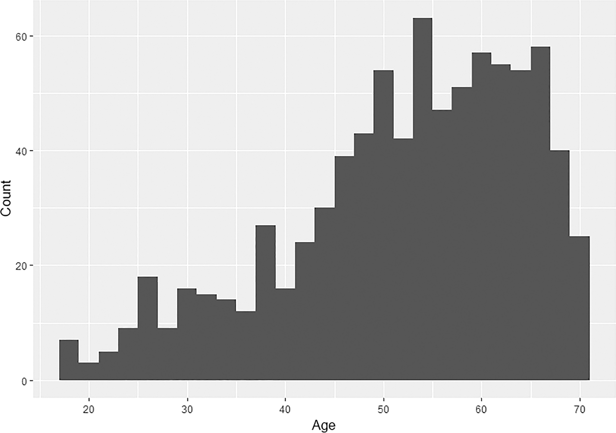
The data consist of 24 standard limb measurements from a total of 833 individuals curated at the William M. Bass Donated Skeletal Collection at the University of Tennessee, Knoxville. Individuals in the current study are predominantly European American adults, ranging in age from 18 to 70 years at death (Fig. 1), a majority of which are male (males = 583, females = 250). The number of individuals varies by comparison, as only those with complete measurements for the compared elements were used.
FIG. 1—Age-at-death distribution of the sample (n = 883).
Methods
Measurements
The measurements used in this study are from the Forensic Anthropology Data Bank (FDB). Some interobserver variability is expected, given the multiple contributors to the FDB. Bivariate plots comparing left- and right-side homologous measurements were used to identify and remove obvious outliers. The number of measurements varies by element (see Table 1). The number and quality of measurements should have an influence on reassociation. Elements with a large number of highly correlated variables should show the highest accuracy rates.
Reassociation Model
This study tests the accuracy of a Bayesian approach to osteometric reassociation by simulating small-scale (n = 10) closed-population commingled assemblages and predicting the best match using standard osteological measurements and Bayesian regression. This process is repeated 500 times for each comparison. Accuracy is defined as the correct classification rate, or the number of times the best match is the correct match divided by 500.
Following Byrd (2008), limb element comparisons are grouped into three types: paired, articulating, and other element comparisons (Table 2). By virtue of being antimeres, measurements are directly comparable between paired elements. For articulating and other comparison types, transformation of raw measurements is required to compare elements.
TABLE 1—Forensic Data Bank Measurements by Element.
|
Element |
Measurement Name |
FDB # |
||
|
Humerus |
Maximum length |
v40 |
||
|
n = 5 |
Epicondylar breadth |
v41 |
||
|
Maximum vertical head diameter |
v42 |
|||
|
Maximum diameter at midshaft |
v43 |
|||
|
Minimum diameter at midshaft |
v44 |
|||
|
Radius |
Maximum length |
v45 |
||
|
n = 3 |
A/P diameter at midshaft |
v46 |
||
|
Transverse diameter at midshaft |
v47 |
|||
|
Ulna |
Maximum length |
v48 |
||
|
n = 4 |
Dorso-Volar diameter |
v49 |
||
|
Transverse diameter |
v50 |
|||
|
Physiological length |
v51 |
|||
|
Femur |
Maximum length |
v60 |
||
|
n = 8 |
Bicondylar length |
v61 |
||
|
Epicondylar breadth |
v62 |
|||
|
Maximum diameter of head |
v63 |
|||
|
A/P subtrochanteric diameter |
v64 |
|||
|
Transverse subtrochanteric diameter |
v65 |
|||
|
A/P diameter at midshaft |
v66 |
|||
|
Transverse diameter at midshaft |
v67 |
|||
|
Tibia |
Condylar-malar length |
v69 |
||
|
n = 4 |
Maximum proximal epiphyseal breadth |
v70 |
||
|
Distal epiphyseal breadth |
v71 |
|||
|
Maximum diameter at nutrient foramen |
v72 |
TABLE 2—Osteometric Comparisons by Type.
|
Comparison |
Type |
|
|
Femur/Femur |
Paired |
|
|
Humerus/Humerus |
Paired |
|
|
Radius/Radius |
Paired |
|
|
Tibia/Tibia |
Paired |
|
|
Ulna/Ulna |
Paired |
|
|
Femur/Tibia |
Articulating |
|
|
Humerus/Ulna |
Articulating |
|
|
Humerus/Radius |
Articulating |
|
|
Ulna/Radius |
Articulating |
|
|
Femur/Humerus |
Other |
|
|
Femur/Ulna |
Other |
|
|
Femur/Radius |
Other |
|
|
Tibia/Humerus |
Other |
|
|
Tibia/Ulna |
Other |
|
|
Tibia/Radius |
Other |
Partial Least Squares
Partial least squares (PLS) analysis is a class of techniques for data reduction and latent variable analysis (Boulestiex & Strimmer 2006; Chen & Hoo 2011; Haenlein & Kaplan 2004; Rosipal & Krämer 2006; Wegelin 2000). These techniques share a common method of extracting components—via ordinary least squares regression. PLS analysis is similar to principal component analysis (PCA) and canonical correlation analysis (CCA), which extract orthogonal (uncorrelated) score vectors that are weighted composites of the original data set (Rosipal & Krämer 2006). Typically, the goal with any type of predictive data reduction analysis is twofold: (1) to find linear combinations that well represent the original variables and (2) to find highly correlated linear combinations. Because PCA captures a maximum amount of variation from the original variables, it is an optimal solution to the first goal. In a predictive framework, where one block of variables is used to predict another block, PCA fails to achieve the second goal, because components between blocks of variables have no relationship. On the other hand, CCA optimally achieves the second goal by creating linear combinations of each block that are maximally correlated with one another. However, CCA fails at the first goal because these components are not designed to capture information or variance within a block and are based on the correlation matrix of raw variables, obscuring the biological meaning of components and making the interpretation of components difficult (Bookstein 1991; Wegelin 2000). Furthermore, CCA components are unstable in instances of multicollinearity, and solutions are not uniquely defined when the number of variables is large compared to the sample size (Wegelin 2000). Simply, PCA explains variation within a block of variables and CCA explains variation between two blocks of variables. While not optimal, PLS achieves both goals by finding linear combinations of variables through the covariance of raw variables that both capture variability and are highly correlated (Bookstein 1991; Wegelin 2000). Components of the X-block (independent variables) are orthogonal, are good representations of X, and are good at explaining Y (dependent variables). Components of the Y-block are orthogonal, are good representations of Y, and are highly correlated with the X-block components. Stated another way, PLS models create components that predict a set of dependent variables from a set of independent variables that have the best predictive power on the dependent variables (Chen & Hoo 2011). The package “plsdepot” (Sanchez 2016) was used in R (R Core Team 2015) to extract relevant PLS components.
Simulated Commingling
Ten individuals were randomly removed from the total data set. These 10 individuals act as a simulated commingled assemblage. One element is chosen as the independent (x) variable, with the 10 possible matching elements acting as the dependent (y) variable. For example, if we are interested in reassociating a left femur with 10 possible right femora, then the left femur is predicting the right femur. In this situation, the left femur is the independent variable and the right femur is the dependent variable. A left femur is selected from the commingled assemblage and compared to the 10 possible right femur matches. These comparisons are made using the model described below, with the remaining sample (total sample excluding the commingled individuals) acting as training data.
Bayesian Regression
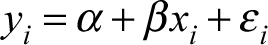
The model used for assessing each variable is a simple linear regression, which takes the form of:
where yi and xi are the ith case of the dependent and independent variables, respectively. The y-intercept is represented by α (alpha), and β (beta) represents the slope, or coefficient by which the independent variable changes in relation to the dependent variable. The error term is εi (sigma) and represents the stochastic part of the model that accounts for all other factors that influence the value of the dependent variable. The y-intercept and slope are the deterministic portions of the model.
Typically, the regression line is fit by finding the line that minimizes the squared vertical distance between all data points. Although point estimates for the y-intercept and slope are calculated, uncertainty is not incorporated into those estimates. Confidence and prediction intervals attempt to deal with this limitation but are often misinterpreted and misapplied. Linear regression of this type is associated with frequentist inference and does not provide an intuitive or easily interpretable way for comparing multiple possible values of yi. Bayesians specify regression models in terms of probability distributions, eliminating these inferential limitations. Bayes’ theorem is used to specify probability distributions, taking the form of:
In this un-normalized form, the posterior probability ρ (θ |y,x) of parameter, θ, given data, y, and constant, x, is proportional (for fixed y and x) to the product of the likelihood function ρ (y|θ,x) and prior ρ (θ,x) (Stan Development Team 2016).
The Bayesian regression model used in this study assigns a normal distribution to the y-variable, with improper (uniform) prior distributions for regression parameters. Unbounded (–∞ to +∞) uniform priors are assigned to the alpha and beta regression parameters, with a positive uniform (0< to +∞) assigned to sigma. These uniform priors are essentially non-informative, leading the posterior distribution of the regression parameters to be driven by the likelihood of the training data. While on its face this model may seem suboptimal by assigning non-informative prior distributions to the regression model, on a practical level this model is needed because of its flexibility. Variable values will change based on the type of comparison and the variable values of the individuals in the training set. Thus, an abstracted regression model is needed to help ensure that predictions are realistic for all variables.
Markov Chain Monte Carlo
Bayesians view parameters as observed realizations of random variables drawn from a probability distribution. As such, parameters are modeled as distributions. Modeling parameters as distributions requires calculus, and calculus is difficult, even for computers. This difficulty and the associated computational modeling time is reduced through Markov chain Monte Carlo (MCMC) simulation. MCMC methods provide a means for exploring the parameter space utilizing equation 2. Given a model, a likelihood, and data, MCMC simulates draws from the posterior distribution using quasi-dependent sequences of random variables (Kéry 2010; S. M. Lynch 2007). This process is repeated a large number of times to approximate the posterior distribution of the parameter, or parameter space.
Many algorithms are available for searching this parameter space. All of them require an initial burn-in or warmup period (Kéry 2010; S. M. Lynch 2007; Stan Development Team 2016). This period is the initial sequence of random draws that are strongly influenced by initial starting values and are not representative of the posterior distribution of the parameter (S. M. Lynch 2007). The Markov chain is considered representative of the posterior parameter space once the chain has converged to equilibrium, or entered a high probability area of the stationary distribution of the parameter (Stan Development Team 2016).
The effectiveness of a MCMC algorithm is measured by its ability to quickly reach convergence and exhaustively explore the parameter space. Many algorithms are inefficient in these respects because they can rely heavily on initial starting values and incoherently search parameter space (Carpenter et al. 2017). Hamiltonian Monte Carlo sampling, however, is both coherent and efficient (Carpenter et al. 2017). This method is based on modeling the behavior of particles using the properties of physical system (Hamiltonian) dynamics (Carpenter et al. 2017; Neal 2011). This system state consists of the position of the particle, q, and the momentum of the particle, p (Neal 2011). The position and momentum of the particle are described by its potential and kinetic energy, respectively (Neal 2011). These energy forms are inversely related. As this particle moves across a surface, its potential and kinetic energy change with the slope of the surface.
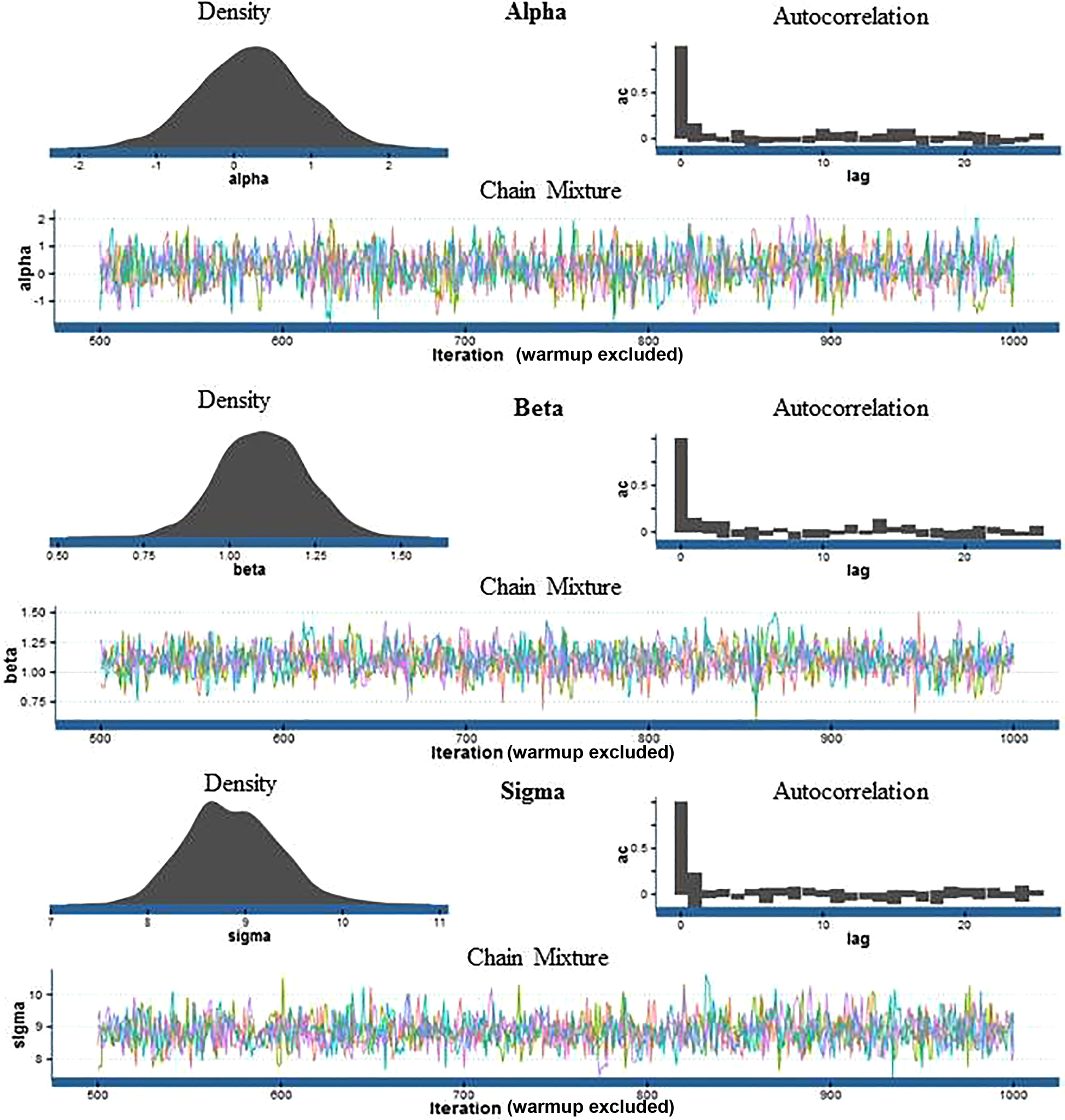
Hamiltonian dynamics are extended to searching parameter space by interpreting the parameter, θ, as the position of a fictional particle at a point in time, with a potential energy defined by the negative log of the probability density of θ and a stochastic momentum variable (Neal 2011; Stan Development Team 2016). Stated simply, Hamiltonian MCMC is an efficient and effective way of exploring parameter space, allowing for the explicit modeling of uncertainty in parameter estimates, including the dependent variable. Thus, instead of a point estimate for an expected bone value, Hamiltonian MCMC provides a distribution of values. These values are weighted by their relative simulated frequency. Convergence of the MCMC simulations is required for the simulated y-values to be a good predictive representation (Stan Development Team 2016). Visual inspection of autocorrelation and chain mixture plots as well as metrics, including r-hat and effective sample size values, are methods for assessing model convergence used in this study.
The Hamiltonian MCMC sampler STAN implemented with the package “rstan” (Stan Development Team 2016) in R (R Core Team 2015) was used to simulate y-values. Specifically, each variable was modeled using 1,000 iterations across four chains with three simulated y-values per iteration. Four chains of 1,000 iterations was chosen over one chain of 4,000 iterations for several reasons. Chains can be ran in parallel, or simultaneously, increasing computational efficiency and reducing run time. Additionally, chains have random starting values. The convergence and proper mixing of each chain provide another check of correct model behavior. The package “shinystan” (Stan Development Team 2016) was used in R (R Core Team 2015) to periodically assess model diagnostics to confirm proper mixing and Markov chain convergence. The default in STAN is to treat the first half of iterations as the burn-in period (Stan Development Team 2016). Thus, for each variable, 6,000 y-values were simulated. Further treatment is required to normalize these values into a probability density function to assess the relative probabilities of each possible match.
Kernel Density Estimation
Kernel density estimation is a means of estimating a probability density function based on the frequency of sample values (Duong 2007). This family of techniques fits a continuous line to the shape of the data with a kernel and bandwidth. The kernel is a non-negative function centered on zero that integrates to one (Duong 2007). The bandwidth is a free parameter that determines the width of the data range on which the kernel function is fit. A small bandwidth for the data results in an under-smoothed density estimate, containing spurious data artifacts, and is essentially “connecting the dots” between data points. An overly wide bandwidth results in an over-smoothed density and obscures the underlying structure of these data. The bandwidth used in this study approaches an optimal solution for the density estimate by selecting a bandwidth that is the standard deviation of the kernel function (R Core Team 2015). The function density() in the package “stats” (R Core Team 2015) was used in R to fit a kernel density to the simulated y-values.
Estimating Best Matches
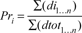
The result of this analysis is a probability density function of y-values for a given x-value for each variable on which the values for the 10 possible matches can be evaluated. The function approx() in the package “stats” (R Core Team 2015) was used in R to evaluate densities for each possible match. These densities are used in two ways to estimate the best match: density weight and equal weight. In the first best match estimate, each possibility is weighted by its density estimate for each variable. This calculation takes the form of:
where Pri is the match probability for the ith possible match, din is the density estimate of the ith possible match for the nth predictive variable, and dtotn is the density estimate of all possible matches for the nth predictive variable. Calculating match probability in this way does not weigh each predictive variable equally. Predictive variables that have high correlations between x-values and y-values will result in tightly dispersed simulated y-values, because uncertainty in its prediction is low (Fig. 2). Conversely, predictive variables that have low correlations also have high uncertainty in y-value predictions, leading to widely dispersed y-values (Fig. 2). This relationship between predictive ability of a variable and the standard error of simulated y-values affects the resulting density estimates (Fig. 3). With this calculation of match probability, predictive variables with higher correlations will lead to higher density estimates and larger relative contributions to the overall match probability. However, these larger relative contributions may swamp the contribution of other, lower correlated variables, leading to spurious classifications if the best match from predictive variables with high correlations is not the correct match.
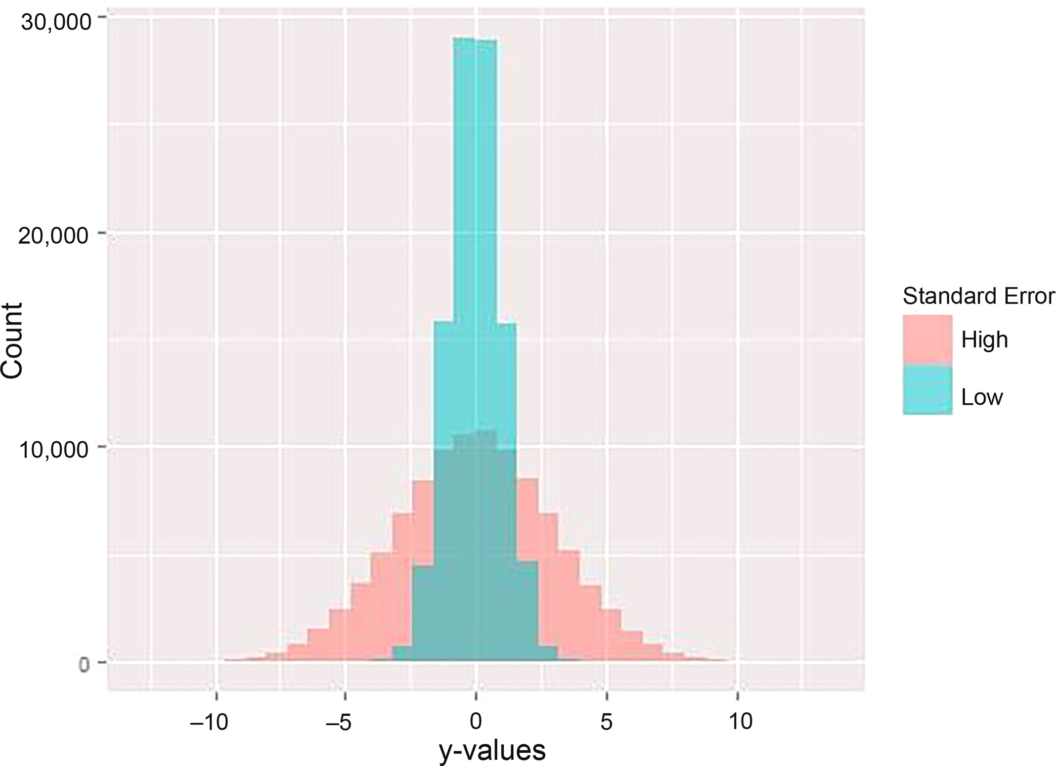
FIG. 2—Relationship between predictive ability of a variable and the distribution of simulated y-values, or the standard error around the mean estimate. Each sample is 100,000 random draws from a normal distribution with a mean of 0 and different standard deviations. The lighter sample (low) has a standard deviation of 1, and the darker sample (high) has a standard deviation of 3.
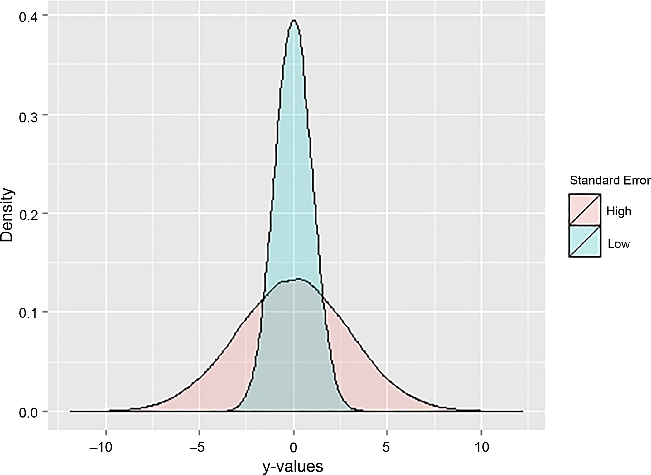
FIG. 3—The density distributions of the samples in Figure 2. A high standard error in the estimation of y results in low density estimates, especially for the mean predicted y-value. Conversely, a low standard error results in high density estimates for values around the mean.
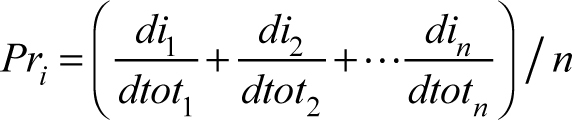
The second calculation of overall match probability weighs all predictive variables equally and takes the form of:
where the notation is the same as formula 3. Here, densities are normalized into probabilities for each variable. The overall match probability is the sum of these probabilities divided by the number of variables. This way of calculating the best match artificially increases the relative importance of variables with low predictive ability. Each method for assessing the best match has possible strengths and weaknesses. Thus, each type is employed to empirically address which performs best.
Quantile Tests
Best match probabilities are a poor metric for recognizing model error. Similar to other methods that classify using Bayesian probability, one of the possible matches will be classified as the best match even when the actual match is not among the possible choices. Thus, it is useful to have another metric by which to assess possible matches. To this end, the 5% and 95% quantiles of the simulated range of y-values were identified. A possible match failed this test if it fell outside of these boundaries. Quantile tests can be interpreted as a two-tailed significance test with an alpha level of 0.10. These tests may be used to reject possible matches, similar to the traditional logic, or to aid in identifying model error. There is a major difference between traditional rejection-based logic, which arrives at a single p-value, and the quantile tests of this study (Adams & Byrd 2006; Byrd 2008; Byrd & Adams 2003; Byrd & LeGarde 2014; J. J. Lynch 2018; Warnke-Sommer et al. 2019). Quantile tests for possible matches were conducted for each variable, with the number of variables ranging from eight for the femur to three for many other comparisons (see Table 1). Quantile tests allow for the examination of this metric as a means of assessing model error and as a rejection criterion. Conducting a quantile test on each variable relates Type 1 error rates to the number of variables rather than directly to the possible match. Thus, comparisons with more variables increase the number of chances for Type 1 error (rejecting a possible match if any variable failed the quantile test). The equation for the expected Type 1 error rate for correct matches is:
where pfail is the expected chance of failing a quantile test and n is the number of variables.
Results
Classification Accuracy
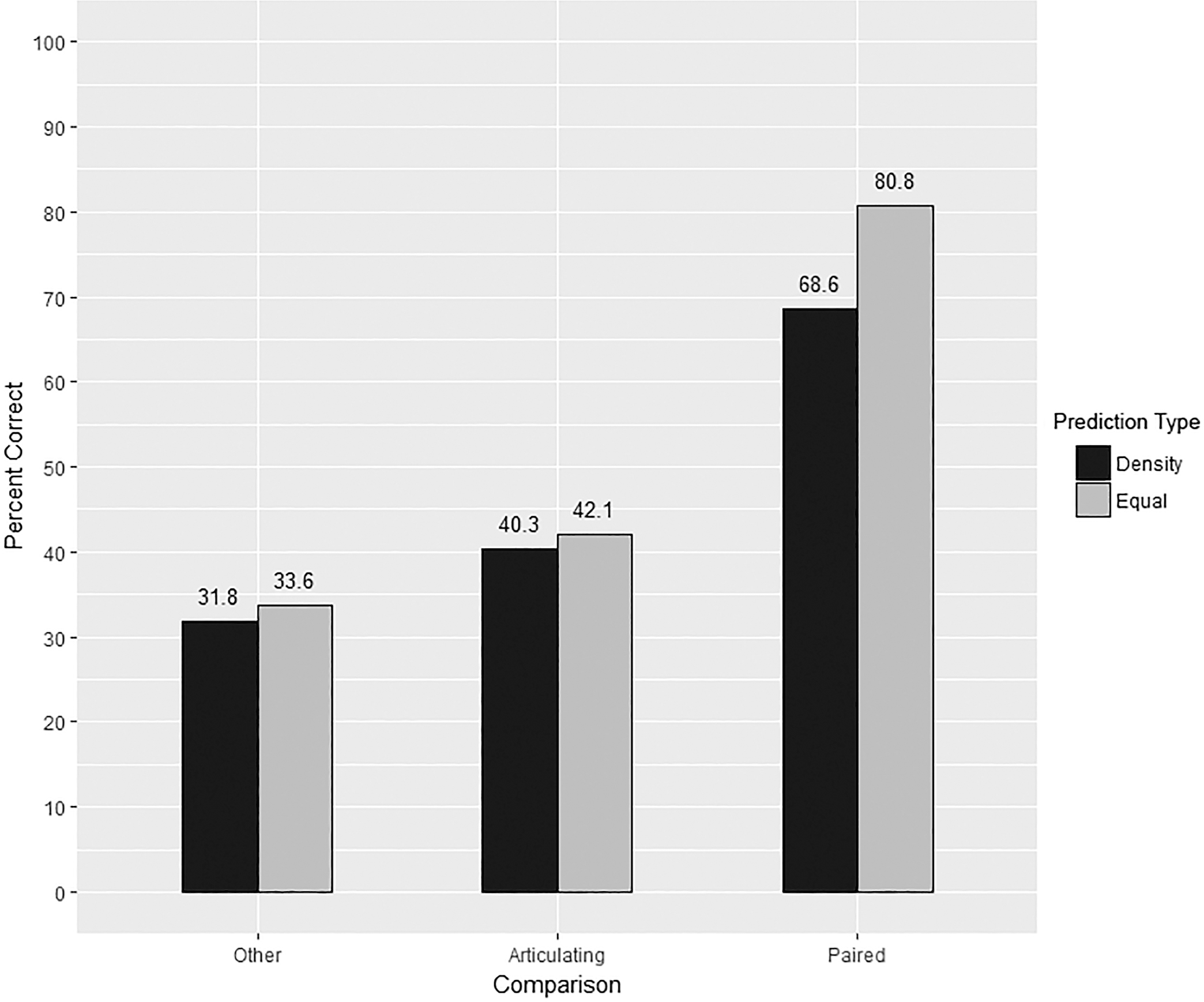
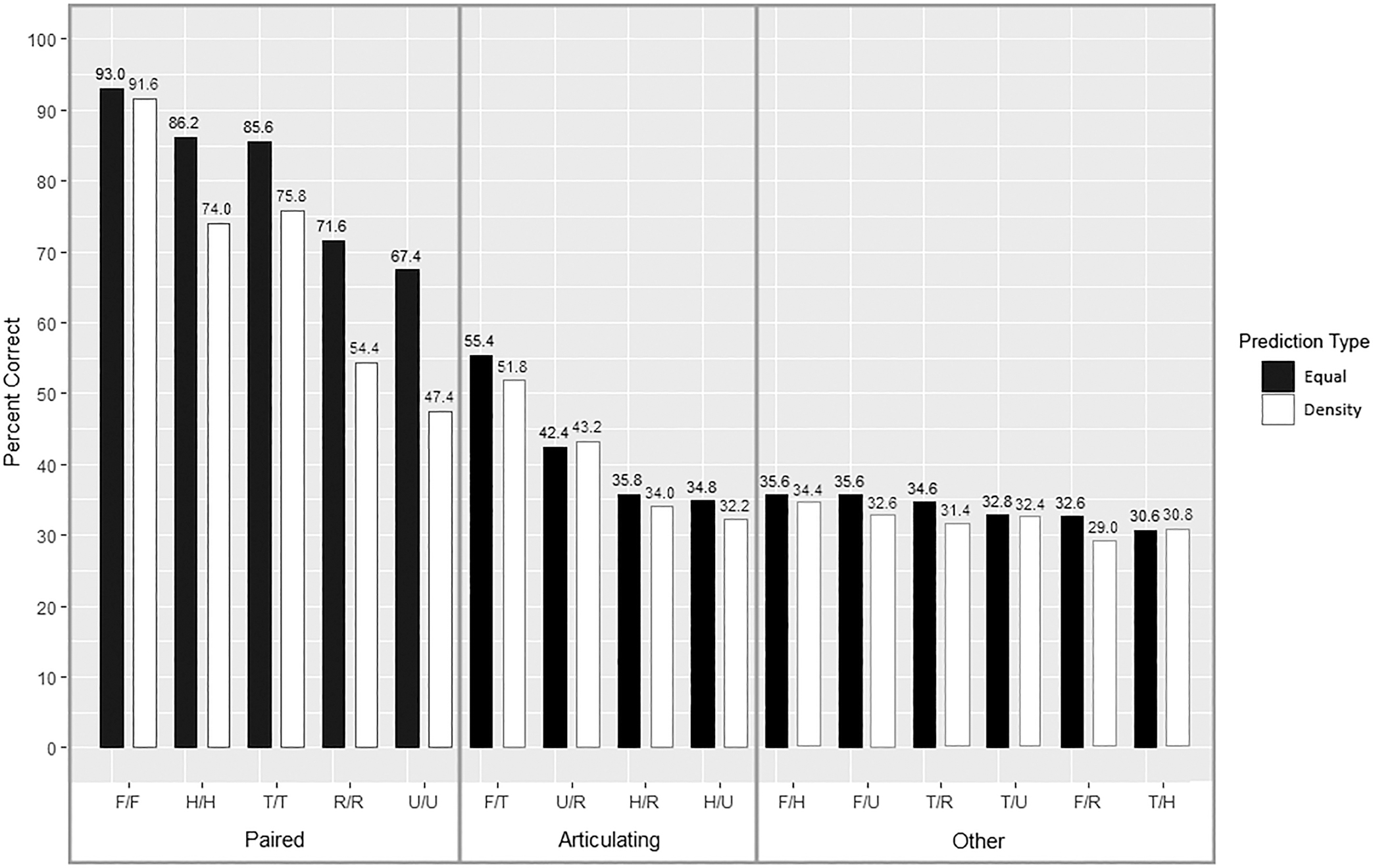
Among all comparison types, the correct match was identified in 51.60% of the simulations (3,870/7,500). Correct classification varied by prediction and comparison types (Fig. 4). In all but two instances, equal-weight comparisons provided the best classification (Table 3 and Fig. 5). With an average difference of 12.12%, paired elements exhibit the largest difference between prediction types. Interestingly, femur/femur equal-weight comparisons only showed a 1.4% improvement. Articulating elements and other comparisons, at an average increase of 1.80% and 1.86%, respectively, showed a minimal difference between prediction types.
FIG. 4—Accuracy by comparison and prediction type.
TABLE 3—Accuracy of Osteometric Comparison Types.
|
Comparison |
Type |
Equal Weight |
Density Weight |
|||
|
Femur/Femur |
Paired |
93.00%* |
91.60% |
|||
|
Humerus/Humerus |
Paired |
86.20% |
74.00% |
|||
|
Tibia/Tibia |
Paired |
85.60% |
75.80% |
|||
|
Radius/Radius |
Paired |
71.60% |
54.40% |
|||
|
Ulna/Ulna |
Paired |
67.40% |
47.40% |
|||
|
Paired Overall |
80.76% |
68.64% |
||||
|
Femur/Tibia |
Articulating |
55.40% |
51.80% |
|||
|
Ulna/Radius |
Articulating |
42.40% |
43.20% |
|||
|
Humerus/Radius |
Articulating |
35.80% |
34.00% |
|||
|
Humerus/Ulna |
Articulating |
34.80% |
32.20% |
|||
|
Articulating Overall |
42.10% |
40.30% |
||||
|
Femur/Humerus |
Other |
35.60% |
34.40% |
|||
|
Femur/Ulna |
Other |
35.60% |
32.60% |
|||
|
Tibia/Radius |
Other |
34.60% |
31.40% |
|||
|
Tibia/Ulna |
Other |
32.80% |
32.40% |
|||
|
Femur/Radius |
Other |
32.60% |
29.00% |
|||
|
Tibia/Humerus |
Other |
30.60% |
30.80% |
|||
|
Other Overall |
33.63% |
31.77% |
||||
|
Overall |
51.60% |
46.33% |
*Bold indicates prediction types with the highest correct classification rates.
FIG. 5—Accuracy of all osteometric comparisons by prediction type.
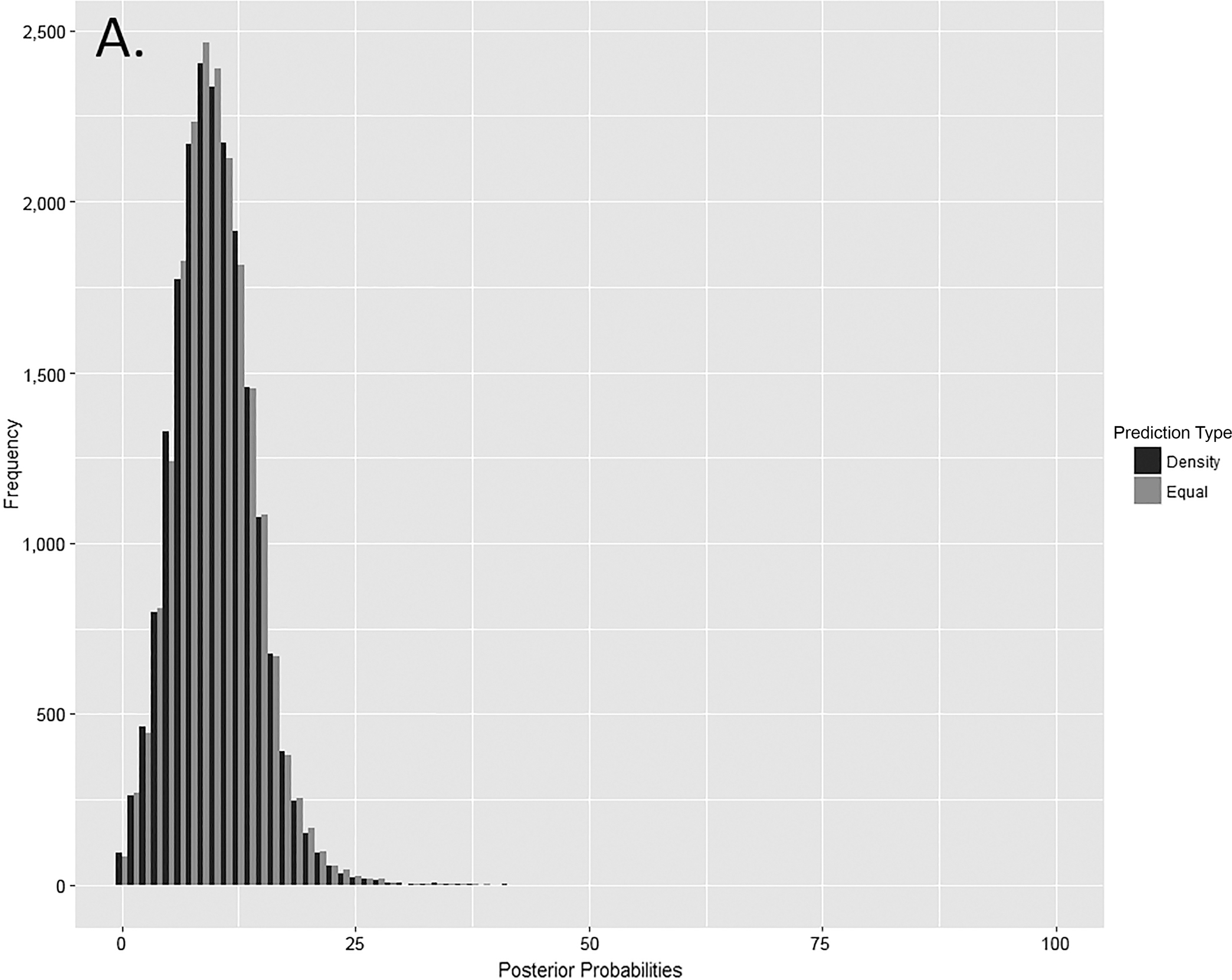
Differences in prediction type should be identifiable through the distribution of posterior probabilities. The distributions of density and equal-weight posterior probabilities are quite similar (Fig. 6). Moreover, the differences between median values for equal-weight and density predictions are negligible (0.08% for other elements, 0.13% for paired elements, and 0.23% for articulating elements). The strong similarities in prediction type distributions for paired elements are unexpected given the difference in accuracy. Given the better or similar classification and similar distributional properties, correct classification refers to equal-weight predictions unless otherwise specified.
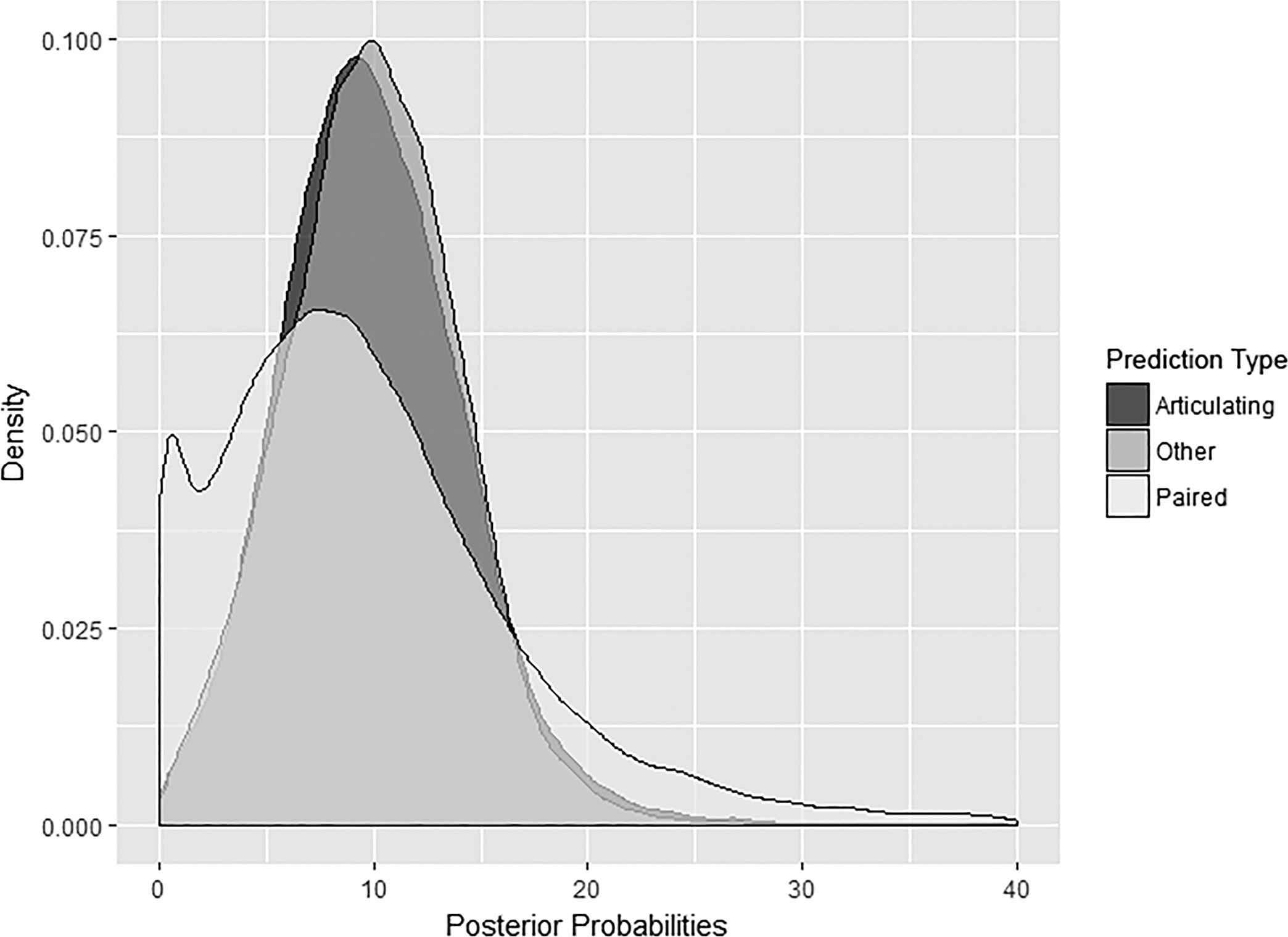
Paired elements performed markedly better than the two other comparison types, almost doubling the accuracy of articulating elements. In contrast, the difference between articulating and other comparisons was less than 10% (see Table 2). Unlike prediction type, the distribution of posterior probabilities by comparison type shows distinct differences (Fig. 7). The relatively low accuracies of articulating and other element comparisons result in slightly positively skewed normal distribution. Paired elements, on the other hand, show a bimodal distribution with a strong positive skew. The shape of these distributions is in line with expectations based on comparison type accuracies. The low accuracy of articulating and other comparisons is due to uncertainty. This randomness leads to posterior probabilities approximating a normal distribution over a large number of trials. The high accuracy of paired elements results in less uncertainty. This structure results in a model that not only predicts the best match well but is also good at identifying bad and not-so-bad matches, leading to a high density of values near zero, another peak near the median, and a long positive tail.
Besides identifying the best match, posterior probabilities rank all possible matches. This aspect is most useful when the analyst is trying to cull down possible matches, in open-population situations, or in non-paired comparisons, where correct classification rates are relatively low. Tables 4–6 provide the best match rank of the correct match. For paired element comparisons, the correct match is among the top three best matches in over 97% of the simulations. For articulating and other comparisons, the correct match is among the top five best matches for 85.85% and 81.74% of simulations, respectively.

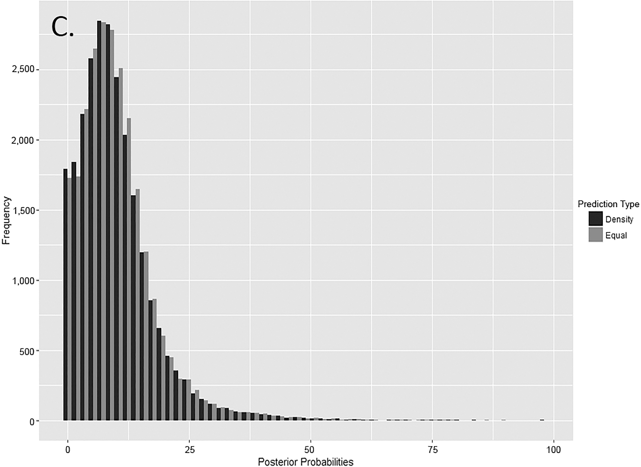
FIG. 6—Distribution of posterior probabilities for (A) other elements (n = 30,000 for each prediction type), (B) articulating elements (n = 20,000 for each prediction type), and (C) paired elements (n = 25,000 for each prediction type).
FIG. 7—Distribution of posterior probabilities for other elements (n = 30,000 for each prediction type), articulating elements (n = 20,000 for each prediction type), and paired elements (n = 25,000 for each prediction type).
Quantile Tests
For each variable, possible match values were compared against the 5% and 95% quantiles of the predicted match distribution, resulting in 300,000 quantile tests. There are interesting trends in the behavior of the quantile tests (Table 7). Correct best match variables failed less often than the expected 10%, with articulating and other comparison variables failing roughly an order of magnitude less. Incorrect best match variables failed more often than correct match variables—10.5% of the time for paired elements, but rarely for articulating and other comparison variables. As expected, variables for other possible matches failed quantile tests more often than best matches. Correct matches failed at least one quantile test (Type 1 error) less than the expected 39.69% for paired, 30.84% for articulating, and 28.37% for other comparisons. Again, Type 1 error for articulating and other comparisons was well below expected rates (see Table 7).
Model Diagnostics
Figure 8 shows an example of typical model diagnostics plot results. These plots show that the MCMC model is working quite well and the parameter estimates are reliable. Density plots should approximate a normal distribution; autocorrelation plots should look like an inverse exponential curve in histogram form, where autocorrelation is initially high and quickly drops off. Chain mixture plots should show no discernible pattern, where each chain moves around parameter space without getting “stuck” in a particular area.
Metric model diagnostics were also periodically checked, including r-hat values and effective sample sizes. An r-hat value is an estimate of convergence based on the mean and standard deviation estimated from each chain (Stan Development Team 2016). Chains have properly converged with r-hat values between 1.0 and 1.2; the closer to 1.0, the better the convergence. Rarely were r-hat values above 1.0, and in no case was an r-hat value above 1.2. Effective sample size is an estimate of the information available from each simulation; the closer the effective sample size is to the number of simulations, the better the chain convergence. Rarely was the effective sample size below 75% of the total number of drawn samples. Most effective sample sizes were between 80 and 90% of the total number of draws, yet another confirmation that model chains are properly converging.
TABLE 4—Paired Element Comparison Correct Match Rank (n = 2,500 Simulations).
|
Rank |
Femur |
Humerus |
Tibia |
Radius |
Ulna |
Total |
% Correct |
Cumulative % |
||||||||
|
1 |
465 |
431 |
428 |
358 |
337 |
2,015 |
80.76 |
80.76 |
||||||||
|
2 |
30 |
50 |
61 |
101 |
107 |
349 |
13.96 |
94.72 |
||||||||
|
3 |
4 |
9 |
6 |
23 |
27 |
69 |
2.76 |
97.48 |
||||||||
|
4 |
0 |
6 |
3 |
5 |
18 |
32 |
1.28 |
98.76 |
||||||||
|
5 |
0 |
1 |
1 |
8 |
8 |
18 |
0.72 |
99.48 |
||||||||
|
6 |
1 |
2 |
0 |
4 |
1 |
8 |
0.32 |
99.80 |
||||||||
|
7 |
0 |
1 |
0 |
0 |
0 |
1 |
0.04 |
99.84 |
||||||||
|
8 |
0 |
0 |
0 |
0 |
1 |
1 |
0.04 |
99.88 |
||||||||
|
9 |
0 |
0 |
1 |
0 |
1 |
2 |
0.08 |
99.96 |
||||||||
|
10 |
0 |
0 |
0 |
1 |
0 |
1 |
0.04 |
100.00 |
TABLE 5—Articulating Element Comparison Correct Match Rank (n = 2,000 Simulations).
|
Rank |
F/T |
U/R |
H/R |
H/U |
Total |
% Correct |
Cumulative % |
|||||||
|
1 |
277 |
212 |
179 |
174 |
842 |
42.10 |
42.10 |
|||||||
|
2 |
102 |
98 |
98 |
89 |
387 |
19.35 |
61.45 |
|||||||
|
3 |
50 |
65 |
80 |
74 |
269 |
13.45 |
75.90 |
|||||||
|
4 |
17 |
36 |
36 |
36 |
125 |
6.25 |
81.15 |
|||||||
|
5 |
15 |
19 |
30 |
30 |
94 |
4.70 |
85.85 |
|||||||
|
6 |
15 |
16 |
14 |
25 |
70 |
3.50 |
89.35 |
|||||||
|
7 |
7 |
14 |
16 |
21 |
58 |
2.90 |
92.25 |
|||||||
|
8 |
6 |
12 |
18 |
13 |
49 |
2.45 |
94.70 |
|||||||
|
9 |
5 |
12 |
15 |
17 |
49 |
2.45 |
97.15 |
|||||||
|
10 |
6 |
16 |
14 |
21 |
57 |
2.85 |
100.00 |
F = femur, H = humerus, T = tibia, R = radius, U = ulna.
TABLE 6—Other Element Comparison Correct Match Rank (n = 3,000 Simulations).
|
Rank |
F/H |
F/U |
F/R |
T/H |
T/U |
T/R |
Total |
% Correct |
Cumulative % |
|||||||||
|
1 |
178 |
178 |
163 |
153 |
164 |
173 |
1,009 |
33.63 |
33.63 |
|||||||||
|
2 |
109 |
87 |
71 |
96 |
94 |
99 |
556 |
18.53 |
52.16 |
|||||||||
|
3 |
73 |
53 |
63 |
84 |
71 |
48 |
392 |
13.07 |
65.23 |
|||||||||
|
4 |
35 |
42 |
72 |
69 |
48 |
54 |
320 |
10.67 |
75.90 |
|||||||||
|
5 |
22 |
36 |
40 |
36 |
39 |
27 |
200 |
6.67 |
82.57 |
|||||||||
|
6 |
19 |
21 |
10 |
23 |
18 |
19 |
110 |
3.37 |
85.94 |
|||||||||
|
7 |
23 |
24 |
17 |
21 |
23 |
21 |
129 |
4.30 |
90.24 |
|||||||||
|
8 |
20 |
16 |
22 |
7 |
20 |
21 |
106 |
3.53 |
93.77 |
|||||||||
|
9 |
11 |
13 |
17 |
7 |
13 |
19 |
80 |
2.67 |
96.44 |
|||||||||
|
10 |
10 |
30 |
25 |
4 |
10 |
19 |
98 |
3.27 |
100.00 |
F = femur, H = humerus, T = tibia, R = radius, U = ulna.
TABLE 7—Quantile Test Results for All Measurements and by Individual.
|
Type |
Position |
Tests |
Fails |
% |
Individuals |
Ind. Fails |
% |
|||||||
|
Paired |
Best/Correct |
14,047 |
640 |
4.56 |
2,019 |
514 |
25.46 |
|||||||
|
Best/Incorrect |
2,953 |
310 |
10.50 |
481 |
48 |
41.16 |
||||||||
|
Other Possibilities |
108,000 |
66,349 |
61.43 |
22,500 |
21,686 |
96.38 |
||||||||
|
Articulating |
Best/Correct |
4,666 |
56 |
1.20 |
842 |
198 |
5.70 |
|||||||
|
Best/Incorrect |
6,334 |
107 |
1.69 |
1,158 |
97 |
8.38 |
||||||||
|
Other Possibilities |
63,000 |
19,105 |
30.33 |
18,000 |
13,158 |
73.10 |
||||||||
|
Other |
Best/Correct |
5,193 |
40 |
0.77 |
1,009 |
34 |
3.39 |
|||||||
|
Best/Incorrect |
10,307 |
116 |
1.28 |
1,991 |
104 |
5.21 |
||||||||
|
Other Possibilities |
85,500 |
23,639 |
27.65 |
27,000 |
17,452 |
64.64 |
||||||||
|
Total |
300,000 |
110,362 |
36.79 |
75,000 |
53,291 |
71.05 |
FIG. 8—An example of typical model diagnostics. The density plot visualizes the posterior distribution of a parameter. The autocorrelation bar graph represents the correlation or dependency of MCMC draws. The chain mixture or trace plot measures how well the sampler is exploring parameter space.
Discussion
The strength of a Bayesian approach to resolving commingling is its versatility. The posterior distribution of y-values allows for the prediction of the correct match and rejecting possible matches. Like most practical applications in forensic anthropology, the analyst must have a clear question to address and a strong understanding of the strengths and weaknesses of the method employed. This study represents a start to understanding those methodological aspects of a Bayesian approach to resolving commingling.
Equal-weight variable predictions perform better than density-weighted predictions. A more nuanced look at trends between prediction types, however, suggests underlying factors that may be affecting classification accuracy by type: the number, type, and predictive ability of measurements (Table 8). As expected, the more highly correlated variables used in the model, the better the accuracy. This trend may explain the almost nonexistent difference between prediction types for the femur and the large difference for other paired comparisons, like the radius. The correlations between left and right length measurements are the strongest for all elements, and are likely driving density-weighted predictions. For the radii, besides maximum length, there are only two moderately correlated measurements of the midshaft. Midshaft measurements are swamped by length in density-weighted comparisons, but are able to adjust the best match to the correct match often in equal-weight predictions. In femur comparisons, the other strongly correlated variables are able to adjust predictions when length-based predictions are wrong, leading to comparable accuracy between the two types. This trend also suggests measurements that quantify different aspects of a bone increase model performance. A likely reason for the high correct classification rates of the femur is the novel information provided by femur measurements. Stated another way, if maximum length is in the model, the addition of bicondylar length is unlikely to appreciably improve performance, as these measurements are, at least statistically, essentially the same (r2 = 0.995). Adding information on epipcondylar breadth, femoral head size, and subtrochanteric dimensions is likely to show a marked increase in model performance at each step. Directly testing this assertion is an avenue for future research.
TABLE 8—Descriptive Statistics of the Correlation between Variables.
|
Comparison |
Type |
# of Vars. |
Avg. r |
Max. r |
Min. r |
|||||
|
Femur/Femur |
Paired |
8 |
0.923 |
0.988 |
0.852 |
|||||
|
Tibia/Tibia |
Paired |
4 |
0.863 |
0.980 |
0.755 |
|||||
|
Humerus/Humerus |
Paired |
5 |
0.840 |
0.964 |
0.722 |
|||||
|
Radius/Radius |
Paired |
3 |
0.792 |
0.964 |
0.671 |
|||||
|
Ulna/Ulna |
Paired |
4 |
0.765 |
0.958 |
0.485 |
|||||
|
All Paired |
24 |
0.837 |
||||||||
|
Femur/Tibia |
Articulating |
4 |
0.646 |
0.910 |
0.306 |
|||||
|
Humerus/Ulna |
Articulating |
3 |
0.593 |
0.778 |
0.344 |
|||||
|
Ulna/Radius |
Articulating |
3 |
0.532 |
0.898 |
0.096 |
|||||
|
Humerus/Radius |
Articulating |
4 |
0.505 |
0.838 |
0.079 |
|||||
|
All Articulating |
14 |
0.569 |
||||||||
|
Tibia/Humerus |
Other |
3 |
0.597 |
0.823 |
0.346 |
|||||
|
Femur/Humerus |
Other |
4 |
0.574 |
0.866 |
0.307 |
|||||
|
Tibia/Ulna |
Other |
3 |
0.551 |
0.775 |
0.175 |
|||||
|
Tibia/Radius |
Other |
3 |
0.540 |
0.779 |
0.133 |
|||||
|
Femur/Ulna |
Other |
3 |
0.508 |
0.778 |
0.155 |
|||||
|
Femur/Radius |
Other |
3 |
0.501 |
0.809 |
0.114 |
|||||
|
All Others |
19 |
0.545 |
||||||||
At an overall performance of just over 50%, it would appear that a Bayesian approach to osteometric reassociation is impractical in many situations. It is important to consider the difficulty of the question that these models are attempting to answer: What is the best match from among these ten possibilities? This question is an order of magnitude more difficult than the question typically asked in osteometric reassociation: Is this one possible match different enough that it can be reliably rejected as a possibility? In this light, an overall performance of just over 50% does not seem so bad. The overall correct classification rate, however, is a misleading metric that obscures some important aspects of osteometric reassociation identified in this study.
Paired element comparisons are superior to articulating and other comparison types. Femora, for example, were correctly matched in 93% of simulations. Paired elements are developmentally and (to varying degrees) functionally integrated elements with directly comparable measurements. Composite variables are required to directly compare non-paired elements. While composite variables are orthogonal and there is a good degree of redundancy by treating each paired element measurement as independent, composite variables are likely obscuring important size and shape relationships that paired element models are able to exploit. This assertion is supported by the lower percentage of quantile rejections for articulating and other type comparisons, where the composite variables may artificially make elements more homogeneous. The use of composite variables should have the largest negative effect in osteometric models based on a rejection criterion. Issues identified in rejection-based osteometric reassociation models (LeGarde 2012; McCormick 2016; Vickers et al. 2015) have been mitigated in recent improvements to and expansions on the paired element model described by Byrd (2008) (J. J. Lynch et al. 2018; Warnke-Sommer et al. 2019). While these changes improve model performance, the underlying logic of the approach has remained the same since its description in Byrd and Adams (2003).
The behavior of quantile tests in this study suggests that deriving one composite p-value as a rejection criterion would be of little value outside of paired element comparisons. Indeed, recent research has focused exclusively on paired element comparisons (J. J. Lynch 2018; J. J. Lynch et al. 2018; Warnke-Sommer et al. 2019). Rejecting a possible match, and by extension, identifying model error for best matches, if any variable failed a quantile test appears to be a viable approach for articulating and other comparisons. This assertion does not apply to paired element comparisons. Over 41% of incorrect best matches and 96% of non-best possibilities fail at least one quantile test, which seems excellent for identifying model error and rejecting possible matches. However, over 25% of the correct best matches also fail at least one quantile test. Despite being below the expected Type 1 error rate (39.69%), it is an unacceptably high rate compared to an aggregate p-value. These results suggest the traditional rejection-based approach is optimal for paired elements.
Conclusions
This study simulated 7,500 closed-population commingled assemblages and assessed the accuracy of predicting the correct match using a complete set of limb measurements. The correct match was identified in 3,870 of the simulations, for an overall correct classification of 51.60%. There are several factors to consider when interpreting the results of this study. The sample used to construct the Bayesian regression model should be near-identical to the average simulated commingled assemblage. While the simulated commingled assemblage was removed from the overall sample prior to the construction of the model, the ten random individuals were drawn from the same population of predominantly European American males. Drawing the commingled assemblage from the same population as the reference sample should have two main influences on these results. First, the reference sample used to create the regression model is very appropriate for the commingled assemblage and represents a “best case” for predicting the best match. Second, the simulated commingled assemblages are, on average, quite homogeneous, making discriminating among possible matches difficult. The relative influence of these factors is beyond the scope of this study. Reference sample composition and homogeneity of the commingled assemblage are additional areas of future research. Other areas of future research include examining the effect of assemblage size, missing measurements, and different methods of quantifying skeletal elements on classification rates.
The reassociation model described above is firmly placed within a Bayesian framework, in both model construction and inference. A Bayesian understanding of probability is easily interpreted and is in line with practical applications of forensic anthropology, where deductive reasoning is required to make statements about a particular case based on a larger theory of knowledge. This approach is not to say the frequentist paradigm is not without merit. In fact, this study has a major aspect that most frequentists would laud—the simulation of commingled assemblages to directly test model performance over the “long run.” The frequency of correct matches over an extended series of trials is an inductive way to build the theoretical foundation on which deductive statements are made. Bayesian modeling is flexible, can be tailored to various types of data, and assumptions can be explicitly built into the model. Modeling parameters as distributions provides an intuitive way to directly compare possible matches. The posterior distribution of y-values can be interpreted in different ways, depending on the goal of the analysis. Although rejecting possible matches has been the purview of the traditional, frequentist approach, there is no reason to limit a Bayesian approach to just prediction. The beauty of the model presented here is the analyst can have the “best of both worlds” through the ability to predict the best match and reject possible matches to create a short list of possibilities. Furthermore, Bayesian inference allows for incorporating additional lines of evidence into the calculation of posterior probabilities. Thus, in theory, other methods or information, such as the spatial relationship between elements recovered in the field, can be incorporated into an overall match probability.
Acknowledgments
The author would like to thank Dr. John Byrd for his mentorship and encouragement to learn more about Bayesian statistics. Thanks are certainly due to Dr. Dawnie Steadman, Dr. Amy Mundorff, Dr. Benjamin Auerbach, Dr. Richard Jantz, and Dr. James Fordyce for their guidance and advice, and to the anonymous reviewers for their thoughtful comments.
References Cited
Adams BJ, Byrd JE, eds. Commingled Human Remains: Methods in Recovery, Analysis, and Identification. San Diego: Academic Press; 2014.
Adams BJ, Byrd JE, eds. Recovery, Analysis, and Identification of Commingled Human Remains. Totowa, NJ: Humana Press; 2008.
Adams BJ, Byrd JE. Resolution of small-scale commingling: A case report from the Vietnam War. Forensic Science International 2006;156(1):63–69.
Bookstein FL. Morphometric Tools for Landmark Data: Geometry and Biology. Cambridge: Cambridge University Press; 1991.
Boulesteix A-L, Strimmer K. Partial least squares: A versatile tool for the analysis of high-dimensional genomic data. Briefings in Bioinformatics 2007;8(1):32–44.
Brennaman AL, Love KR, Bethard JD, Pokines JT. A Bayesian approach to age-at-death estimation from osteoarthritis of the shoulder in modern North Americans. Journal of Forensic Sciences 2017;62(3):573–584.
Buikstra JE, Gordon CC, St. Hoyme L. The case of the severed skull: Individuation in forensic anthropology. In: Rathburn TA, Buikstra JE, eds. Human Identification: Case Studies in Forensic Anthropology. Springfield: Charles C. Thomas; 1984:121–135.
Byrd JE. Models and methods for osteometric sorting. In: Byrd JE, Adams BJ, eds. Recovery, Analysis, and Identification of Commingled Human Remains. Totowa, NJ: Humana Press; 2008:199–220.
Byrd JE, Adams BJ. Analysis of commingled human remains. In: Blau S, Ubelaker DH, eds. Handbook of Forensic Anthropology and Archaeology. Walnut Creek: Left Coast Press; 2009:174–185
Byrd JE, Adams BJ. Osteometric sorting of commingled human remains. Journal of Forensic Sciences 2003;48(4):717–724.
Byrd JE, LeGarde CB. Osteometric sorting. In: Adams BJ, Byrd JE, eds. Commingled Human Remains: Methods in Recovery, Analysis, and Identification. San Diego: Academic Press; 2014;167–191.
Carpenter B, Gelman A, Hoffman MD, Lee D, Goodrich B, Betancourt M, et al. Stan: A probabilistic programming language. Journal of Statistical Software 2017;76(1):1–32. doi: 10.18637/jss.v076.i01
Chen Y, Hoo KA. Application of partial least square regression in uncertainty study area. American Control Conference 2011;1958–1962.
Curtin AJ. Putting together the pieces: Reconstructing mortuary practices from commingled ossuary cremains. In: Schmidt CW, Symes SA, eds. The Analysis of Burned Human Remains. San Diego: Academic Press; 2008;219–227.
Duong T. ks: Kernel density estimation and kernel discriminant analysis for multivariate data in R. Journal of Statistical Software 2007;21(7):1–16.
Gelman A. Objections to Bayesian statistics. Bayesian Analysis 2008;3:445–449.
Haenlein M, Kaplan AM. A beginner’s guide to partial least squares analysis. Understanding Statistics 2004;3(4):283–297.
Herrmann NP, Devlin JB. Assessment of commingled human remains using a GIS-based approach. In: Adams BJ, Byrd JE, eds. Recovery, Analysis and Identification of Commingled Human Remains. Totowa, NJ: Humana Press; 2008;257–269.
Hinkes MJ. The role of forensic anthropology in mass disaster resolution. Aviation, Space, and Environmental Medicine 1989;60:A60–3.
Hoekstra R, Morey RD, Rouder JN, Wagenmakers EJ. Robust misinterpretation of confidence intervals. Psychonomic Bulletin & Review 2014;21(5):1157–1164.
Jantz RL, Ousley SD. FORDISC 3.0: Personal computer forensic discriminant functions. University of Tennessee, Knoxville; 2005.
Kéry M. Introduction to WinBUGS for Ecologists: Bayesian Approach to Regression, ANOVA, Mixed Models and Related Analyses. New York: Academic Press; 2010.
Konigsberg LW, Frankenberg SR. Bayes in biological anthropology. American Journal of Physical Anthropology 2013;152(S57):153–184.
LeGarde CB. Asymmetry of the Humerus: The Influence of Handedness on the Deltoid Tuberosity and Possible Implications for Osteometric Sorting [master’s thesis]. Missoula: University of Montana; 2012.
Lew MJ. To P or not to P: On the evidential nature of P-values and their place in scientific inference stat. arXiv:1311.0081;2013.
Lynch JJ. An analysis on the choice of alpha level in the osteometric pair-matching of the os coxa, scapula, and clavicle. Journal of Forensic Sciences 2018;63(3):793–797.
Lynch JJ, Byrd J, LeGarde CB. The power of exclusion using automated osteometric sorting: Pair-matching. Journal of Forensic Sciences 2018;63(2):371–380.
Lynch SM. Introduction to Applied Bayesian Statistics and Estimation for Social Scientists. New York: Springer Science and Business Media; 2007.
Mayo DG. In defense of the Neyman-Pearson theory of confidence intervals. Philosophy of Science 1981;48(2):269–280.
Mayo DG, Spanos A. Error and Inference: Recent Exchanges on Experimental Reasoning, Reliability, and the Objectivity and Rationality of Science. Cambridge: Cambridge University Press; 2010.
McCormick KA. A Biologically Informed Structure to Accuracy in Osteometric Reassociation [PhD dissertation]. Knoxville: University of Tennessee; 2016.
Mundorff AZ. Anthropologist-directed triage: Three distinct mass fatality events involving fragmentation of human remains. In: Adams BJ, Byrd JE, eds. Recovery, Analysis and Identification of Commingled Human Remains. Totowa, NJ: Humana Press; 2008;123–144.
Mundorff AZ. Integrating forensic anthropology into disaster victim identification. Forensic Science, Medicine, and Pathology 2012;8:131–139.
Neal RM. MCMC using Hamiltonian dynamics. In: Brooks S, Gelman A, Jones GL, Meng X-L, eds. Handbook of Markov Chain Monte Carlo. Boca Raton, FL: CRC Press: 2011:113–162.
O’Brien MJ, Storlie CB. An alternative bilateral refitting model for zooarchaeological assemblages. Journal of Taphonomy 2011;9:245–268.
Primorac D, Andelinovic S, Definis-Gojanovic M, Drmic I, Rezic B, Baden MM, et al. Identification of war victims from mass graves in Croatia, Bosnia, and Herzegovina by the use of standard forensic methods and DNA typing. Journal of Forensic Sciences 1996;41(5):891–894.
R Core Team. R: A language and environment for statistical computing. R Foundation for Statistical Computing, Vienna, Austria, 2015. http://www.R-project.org/.
Rosing FW, Pischtschan E. Re-individualisation of commingled skeletal remains. In: Jacob B, Bonte W, eds. Advances in Forensic Sciences. Berlin: Verlag Dr. Köster; 1995:1–9.
Rosipal R, Krämer N. Overview and recent advances in partial least squares. In: Saunders C, Grobelnik M, Gunn S, Shawe-Taylor J, eds. Subspace, Latent Structure and Feature Selection. Berlin: Springer; 2006:34–51.
Royall R. On the probability of observing misleading statistical evidence. Journal of the American Statistical Association 2000;95(451):760–768.
Royall R. Statistical Evidence: A Likelihood Paradigm. Boca Raton, FL:CRC Press; 1997. Monographs on Statistics and Applied Probability; vol. 71.
Sanchez G. plsdepot: Partial least squares (PLS) data analysis methods. R package version 0.1, 17; 2016.
Sledzik PS, Rodriguez WC. Damnum fatale: The taphonomic fate of human remains in mass disasters. In: Haglund WD, Sorg MH, eds. Advances in Forensic Taphonomy: Method, Theory, and Archaeological Perspectives. Boca Raton, FL: CRC Press; 2001;322–330.
Snow CC, Folk ED. Statistical assessment of commingled skeletal remains. American Journal of Physical Anthropology 1970;32:423–427.
Stan Development Team. Stan modeling language: User’s guide and reference manual, Version 2.17.0; 2016.
Stark PB, Freedman DA. What is the chance of an earthquake? NATO Science Series IV: Earth and Environmental Sciences 2003;32:201–213.
Steadman DW, Sperry K, Snow F, Fulginiti L, Craig E. Anthropological investigations of the Tri-State Crematorium incident. In: Adams BJ, Byrd JE, eds. Recovery, Analysis and Identification of Commingled Human Remains. Totowa, NJ: Humana Press; 2008:81–96.
Ubelaker DH, Rife JL. Approaches to commingling issues in archeological samples: A case study from Roman era tombs in Greece. In: Adams BJ, Byrd JE, eds. Recovery, Analysis and Identification of Commingled Human Remains. Totowa, NJ: Humana Press; 2008:97–122.
Varas CG, Leiva MI. Managing commingled remains from mass graves: Considerations, implications and recommendations from a human rights case in Chile. Forensic Science International 2012;219:e19–e24.
Vickers S, Lubinski PM, DeLeon LH, Bowen JT. Proposed method for predicting pair matching of skeletal elements allows too many false rejections. Journal of Forensic Sciences 2015;60(1):102–106.
Warnke-Sommer JD, Lynch JJ, Pawaskar SS, Damann FE. Z-Transform method for pairwise osteometric pair-matching. Journal of Forensic Sciences. 2019;64(1):23–33.
Wegelin JA. A survey of partia1 least squares (PLS) methods, with emphasis on the two-block case. Technical report, Department of Statistics, University of Washington, Seattle; 2000.
Willey PS. Prehistoric Warfare on the Great Plains: Skeletal Analysis of the Crow Creek Massacre Victims. New York: Garland Publications; 1990.
aDefense POW/MIA Accounting Agency, DoD, Hawai’i, USA
*Correspondence to: Kyle McCormick, Defense POW/MIA Accounting Agency, DoD, 590 Moffett St., Joint Base Pearl Harbor–Hickam, AFB, Hawai’i 96853, USA
E-mail: kmccormick9@yahoo.com
Received 19 June 2018; Revised 17 October 2018; Accepted 26 October 2018
 (1)
(1) (2)
(2) (3)
(3)
 (4)
(4) (5)
(5)